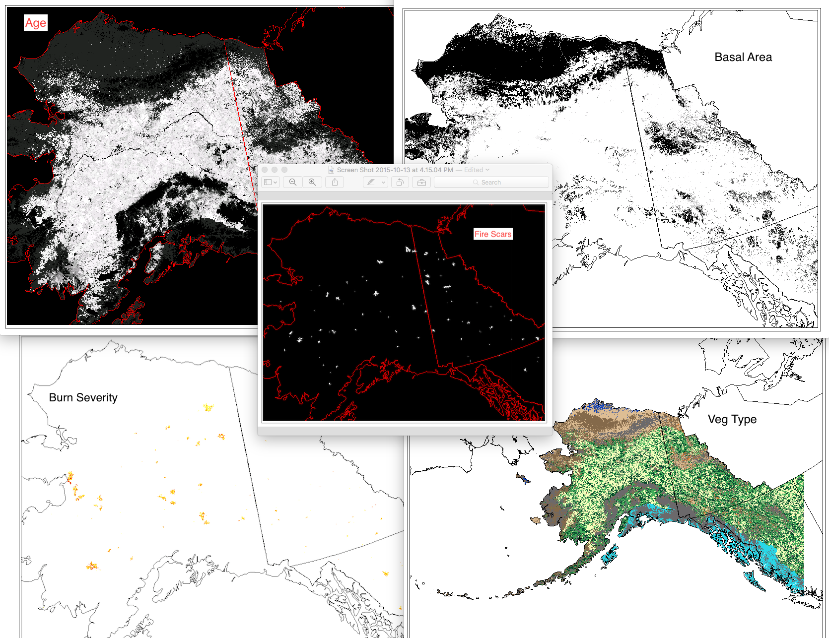
This set of files includes annual model outputs from ALFRESCO, a landscape scale fire and vegetation dynamics model. These specific outputs are from the Integrated Ecosystem Model (IEM) project, and are from the linear coupled version using AR4/CMIP3 climate inputs (IEM Generation 1-AR4) and AR5/CMIP5 climate inputs (IEM Generation 1-AR5). These outputs include data from model rep 171(IEM Generation 1-AR4) and rep 26 (IEM Generation 1-AR5), referred to as the “best rep” out of 200 replicates. The best rep was chosen through comparing ALFRESCO’s historical fire outputs to observed historical fire patterns. Single rep analysis is not recommended as a best practice, but can be used to visualize possible changes. Climate models and emission scenarios: IEM Generation 1-AR4/CMIP3 CCCMA-CGCMS-3.1 MPI-ECHAM5 under the SRES A1B scenario IEM Generation 1-AR5/CMIP5 MRI-CGCM3 NCAR-CCSM4 under RCP 8.5 scenario Variables include: Veg: The dominant vegetation for this cell. Current values are: 0 = Not Modeled 1 = Black Spruce 2 = White Spruce 3 = Deciduous Forest 4 = Shrub Tundra 5 = Graminoid Tundra 6 = Wetland Tundra 7 = Barren / Lichen / Moss 8 = Temperate Rainforest Age: This the age of the vegetation in each cell. An Age value of 0 means it transitioned in the previous year. Basal Area: The accumulation of basal area of white spruce in tundra cell, and is influenced by seed dispersal, growth of biomass, climate data, and other factors. units = m^2 / ha Burn Severity: This is a categorical burn severity level of the previous burn in the current cell, influenced by fire size and slope. For example, a burn severity value in a file with year 1971 in the file name means that the severity level given to that file occurred in the fire that occurred in year 1970. 0=No Burn 1=Low 2=Moderate 3=High w Low Surface Severity 4=High w/ High Surface Severity Fire Scar: These are the unique fire scars. Each cell has three values. Band 1 - Year of burn Band 2 - Unique ID for the simulated fire for that simulation year Band 3 - Whether or not the cell was an ignition location for a fire. There will only be 1 ignition cell per fire per year. 0 = not ignition 1 = ignition point For background on ALFRESCO, please refer to: Is Alaska's Boreal Forest Now Crossing a Major Ecological Threshold? Daniel H. Mann, T. Scott Rupp, Mark A. Olson, and Paul A. Duffy Arctic, Antarctic, and Alpine Research 2012 44 (3), 319-331 http://www.bioone.org/doi/abs/10.1657/1938-4246-44.3.319

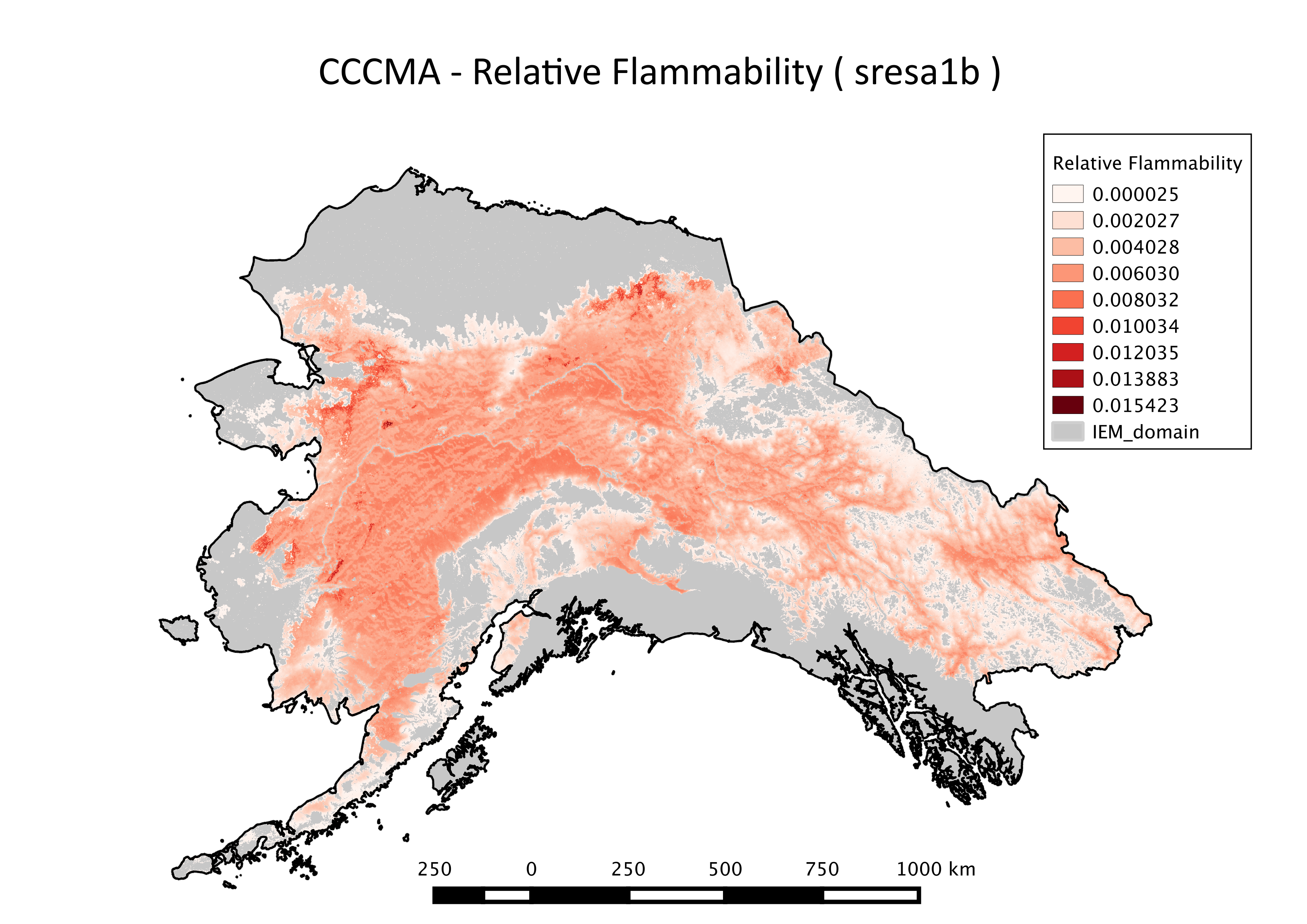
This file includes spatial representations of relative flammability produced through summarization of the ALFRESCO model outputs. These specific outputs are from the Integrated Ecosystem Model (IEM) project, and are from the linear coupled version using AR5/CMIP5 climate inputs (IEM Generation 2). This dataset has been updated to include flammability data summarized over additional time scales as well, done in the same manner as the intial dataset. These ALFRESCO outputs were summarized over three future eras (2010-2039, 2040-2069, 2070-2099) and a historical era (1950-2008), for two future emissions scenarios for five CMIP5 models

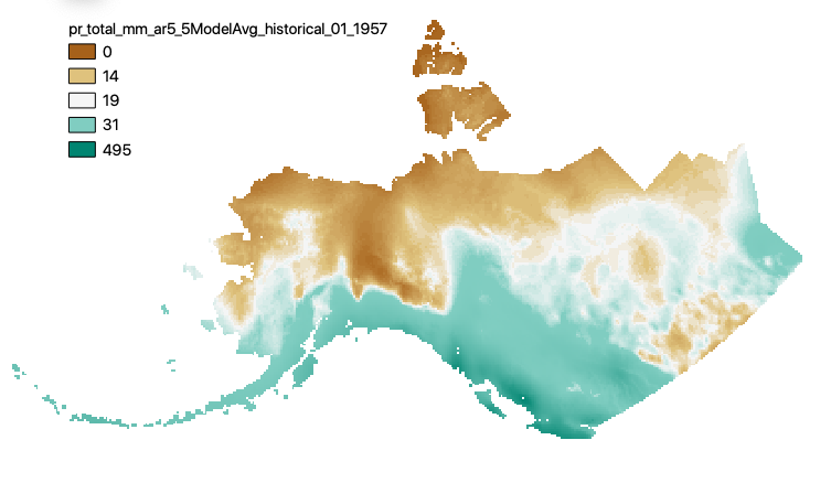
This set of files includes downscaled historical estimates of monthly total precipitation (in mm, no unit conversion necessary) from 1901 - 2005, at 15km x 15km spatial resolution. They include data for Alaska and Western Canada. Each set of files originates from one of five top ranked global circulation models from the CMIP5/AR5 models and RCPs, or is calculated as a 5 Model Average. These outputs are from the Historical runs of the GCMs. The downscaling process utilizes CRU CL v. 2.1 climatological datasets from 1961-1990 as the baseline for the Delta Downscaling method.

This dataset consists of four different variables: degree days below 65°F (or "heating degree days"), degree days below 0°F, degree days below 32°F (or "air freezing index"), and degree days above 32°F (or "air thawing index"). All were derived from the same set of nine statistically downscaled CMIP5 global climate model outputs driven by RCP 4.5 and RCP 8.5 emissions scenarios. A historical baseline (Daymet, 1980-2017) dataset is included for each variable. All data are in GeoTIFF format and have a spatial resolution of 12 km. Units are degree days Fahrenheit (°F⋅days). The model-scenario combinations are: - ACCESS1-3, RCP 4.5 - ACCESS1-3, RCP 8.5 - CanESM2, RCP 4.5 - CanESM2, RCP 8.5 - CCSM4, RCP 4.5 - CCSM4, RCP 8.5 - CSIRO-Mk3-6-0, RCP 4.5 - CSIRO-Mk3-6-0, RCP 8.5 - GFDL-ESM2M, RCP 4.5 - GFDL-ESM2M, RCP 8.5 - inmcm4, RCP 4.5 - inmcm4, RCP 8.5 - MIROC5, RCP 4.5 - MIROC5, RCP 8.5 - MPI-ESM-MR, RCP 4.5 - MPI-ESM-MR, RCP 8.5 - MRI-CGCM3, RCP 4.5 - MRI-CGCM3, RCP 8.5 The .zip files that are available for download are organized by variable. One .zip file has all the models and scenarios and years for that variable. Each GeoTIFF file has a naming convention like this: "ncar_12km_{model}_{scenario}_{variable}_{year}_Fdays.tif" Each GeoTIFF has a 12 km by 12 km pixel size, and is projected to EPSG:3338 (Alaska Albers).

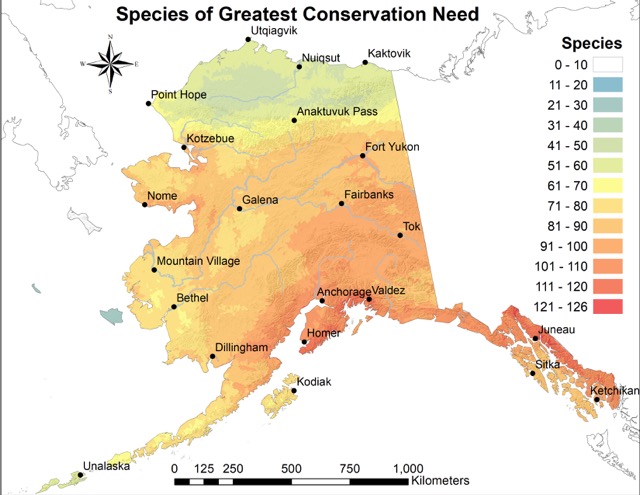
This dataset represents the results of a project that compiled available range information for three taxonomic groups representing 211 species (159 birds, 45 mammals, and 5 amphibians) identified as Species of Greatest Conservation Need (SGCN) by the 2015 Alaska Wildlife Action Plan (SWAP) Appendix A (https://www.adfg.alaska.gov/index.cfm?adfg=wildlifediversity.swap) in addition to 2 amphibian species native to Alaska. The goal of this effort was to create an initial set of statewide heatmaps of SGCN richness. Files include: (1) a set of 21 species richness heat maps depicting the sum of overlapping range maps from multiple SGCNs; (2) shapefiles of species range maps for Alaska’s terrestrial SGCN, with all species ranked (high, moderately high, moderate, low) in terms of relative conservation and management priority based on the Alaska Species Ranking System (ASRS; https://accs.uaa.alaska.edu/wildlife/alaska-species-ranking-system); (3) shapefiles of species in decline for birds and marine mammals (as listed in SWAP Appendix A); and (4) a file that cross-walks each SGCN by species code, common name, and scientific name. Complete information describing how environmental variables correlated with species richness is provided in the final report (http://data.snap.uaf.edu/data/Base/Other/Species/State_Wildlife_Grant_Final_Report_20Sept24.pdf). Species richness maps were derived from species-specific, 6th-level hydrologic unit (HUC12) occupancy maps developed by the Alaska Gap Analysis Project (https://accscatalog.uaa.alaska.edu/dataset/alaska-gap-analysis-project). Hotspot maps highlight all HUCs containing more than 60% of considered amphibian species or 80% of the maximum number of co-occurring bird or mammal species. Species richness values were derived by summing the number of species with overlapping ranges. A gradient boosting machine algorithm quantified relationships between SGCN hotspots and a set of 24 climatic, topographic, and habitat predictors. It is important to note that species ranges are modeled and extrapolated from limited data. They may be affected by changes in our understanding of species' ranges, changes in taxonomy, and changes in what we consider to be the best tools and data for creating distribution models using presence-only data, and may overestimate actual ranges. These datasets and any associated maps and other products are intended to provide a landscape-level overview only. It is highly recommended that any use of these datasets be undertaken in conjunction with expert advice from the Alaska Department of Fish and Game (see contact information below).

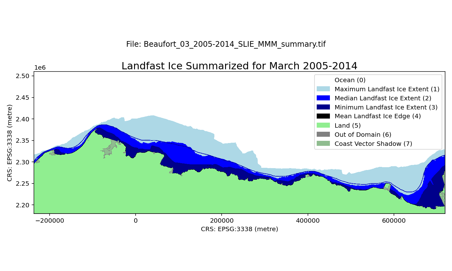
A landfast ice dataset along the Beaufort Sea continental shelf, spanning 1996-2023. Spatial resolution is 100 m. Each month of the ice season (October through July) is summarized over three 9-year periods (1996-2005, 2005-2014, 2014-2023) using the minimum, maximum, median, and mean distance of SLIE from the coastline. The minimum extent indicates the region that was always occupied by landfast ice during a particular calendar month. The median extent indicates where landfast occurred at least 50% of the time. The maximum extent represents regions that may only have been landfast ice on one occasion during the selected time period. The mean SLIE position for the each month and and time period is also included. The dataset is derived from three sources: seaward landfast ice images derived from synthetic aperture radar images from the RadarSAT and EnviSAT constellations (1996-2008), the Alaska Sea Ice Program (ASIP) ice charts (2008-2017, 2019-2022), and the G10013 SIGID-3 Arctic Ice Charts produced by the National Ice Center (NIC; 2017-2019, 2022-2023). Within each GeoTIFF file there are 8 different pixel values representing different characteristics: 0 - Ocean 1 - Maximum Landfast Ice Extent 2 - Median Landfast Ice Extent 3 - Minimum Landfast Ice Extent 4 - Mean Landfast Ice Edge 5 - Land 6 - Out of Domain 7 - Coast Vector Shadow The file naming convention is as follows: Beaufort_$month_$era_SLIE_MMM_summary.tif For example, the name Beaufort_05_2005-2014_SLIE_MMM_summary.tif indicates the file represents data for May 2005-2014. These data were updated on August 21, 2025 to rectify the omission of some NIC chart data sources for the 2017-18 and 2018-19 seasons.

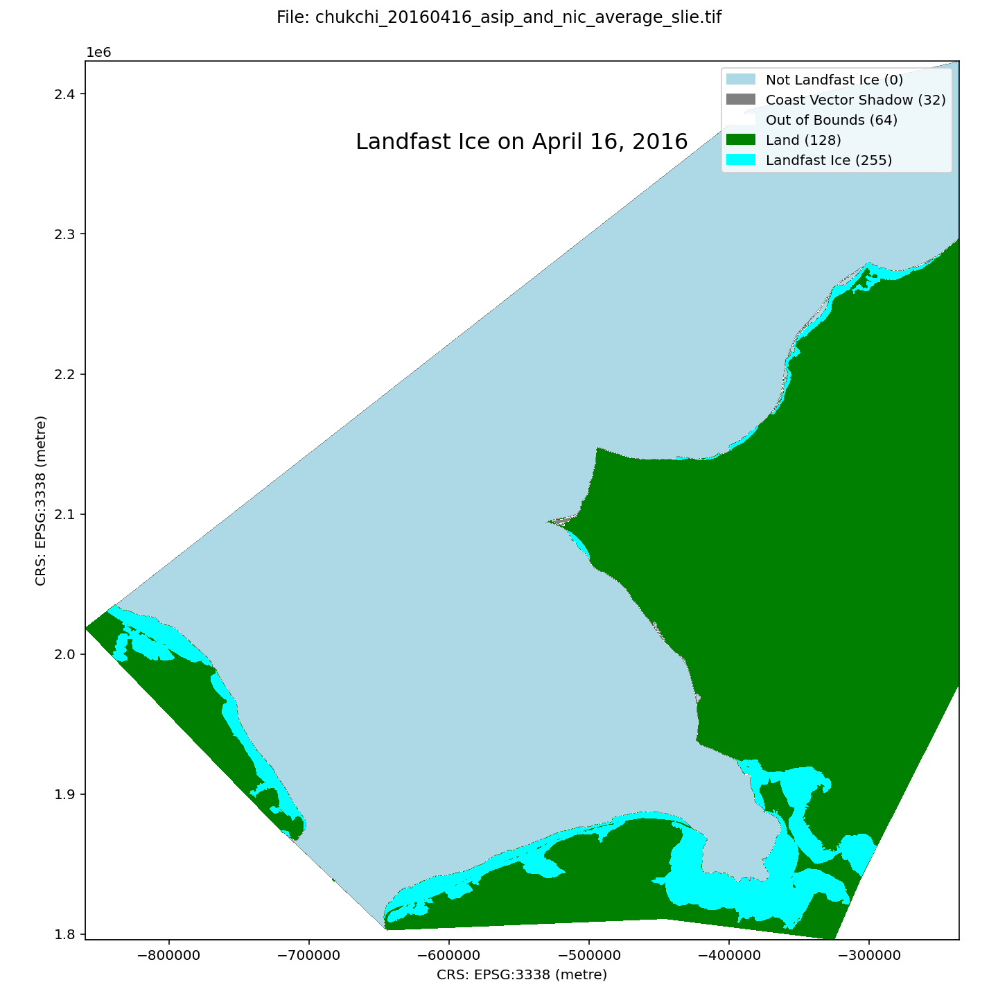
A dataset of landfast ice extent along the Alaska coast of the Chukchi Sea and adjacent waters in Russia, spanning the winters of 1996-2023. Landfast ice extent is defined as the area between the coast and the seaward landfast ice edge (SLIE), meaning that small areas of open water than can form at the coast springtime will not be represented. Spatial resolution is 100 m. Compilation of the dataset is described in detail by Mahoney et al (2024). In brief, it is derived from three sources: From 1996-2008, the dataset is derived from analysis of sequential synthetic aperture radar (SAR) images from the RadarSAT and EnviSAT constellations, as described by Mahoney et al (2014); From 2008-2023, the data represent an average landfast extent identified in ice charts from the U.S. National Weather Service Alaska Sea Ice Program (ASIP) and the U.S. National Ice Center (NIC). Within each GeoTIFF file there are 5 different pixel values representing different characteristics: 0 - Not Landfast Ice 32 - Coast Vector Shadow 64 - Out of Bounds 128 - Land 255 - Landfast ice The file naming convention is as follows: chukchi_$YYYYMMDD_$source_slie.tif For example, the name chukchi_20170302_asip_and_nic_average_slie.tif indicates the file represents data for March 2, 2017 and that the data is derived from an average of the ASIP and NIC data sources. These data were updated on August 21, 2025 to rectify the omission of some NIC chart data sources for the 2017-18 and 2018-19 seasons.

This set of files includes downscaled projections of decadal means of annual day of freeze or thaw (ordinal day of the year), and length of growing season (numbers of days, 0-365) for each decade from 2010 - 2100 at 2km x 2km meter spatial resolution. Each file represents a decadal mean of an annual mean calculated from mean monthly data. ---- The spatial extent includes Alaska, the Yukon Territory, British Columbia, Alberta, Saskatchewan, and Manitoba. Each set of files originates from one of five top ranked global circulation models from the CMIP5/AR5 models and RPCs, or is calculated as a 5 Model Average. Day of Freeze, Day of Thaw, Length of Growing Season calculations: Estimated ordinal days of freeze and thaw are calculated by assuming a linear change in temperature between consecutive months. Mean monthly temperatures are used to represent daily temperature on the 15th day of each month. When consecutive monthly midpoints have opposite sign temperatures, the day of transition (freeze or thaw) is the day between them on which temperature crosses zero degrees C. The length of growing season refers to the number of days between the days of thaw and freeze. This amounts to connecting temperature values (y-axis) for each month (x-axis) by line segments and solving for the x-intercepts. Calculating a day of freeze or thaw is simple. However, transitions may occur several times in a year, or not at all. The choice of transition points to use as the thaw and freeze dates which best represent realistic bounds on a growing season is more complex. Rather than iteratively looping over months one at a time, searching from January forward to determine thaw day and from December backward to determine freeze day, stopping as soon as a sign change between two months is identified, the algorithm looks at a snapshot of the signs of all twelve mean monthly temperatures at once, which enables identification of multiple discrete periods of positive and negative temperatures. As a result more realistic days of freeze and thaw and length of growing season can be calculated when there are idiosyncrasies in the data. Please note that these maps represent climatic estimates only. While we have based our work on scientifically accepted data and methods, uncertainty is always present . Uncertainty in model outputs tends to increase for more distant climatic estimates from present day for both historical summaries and future projections.

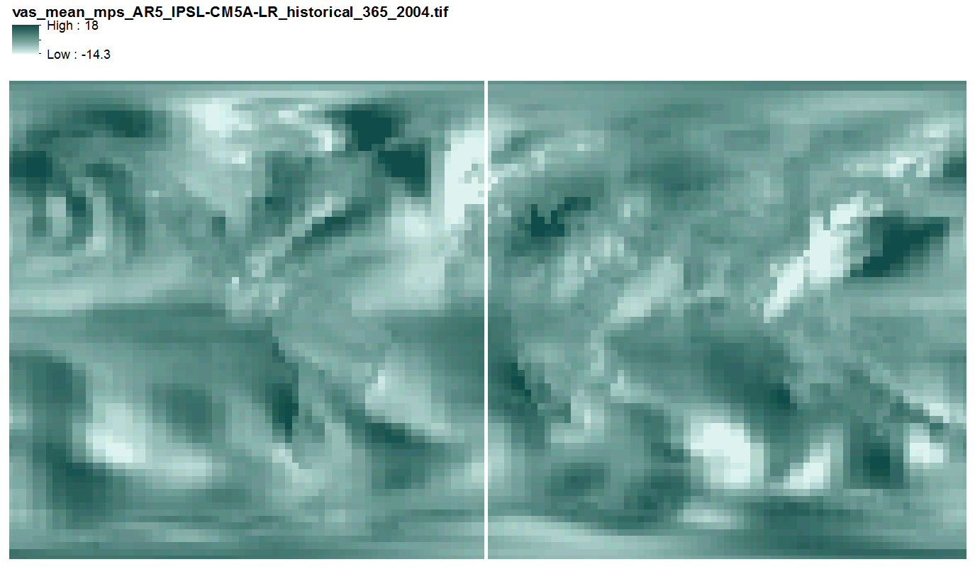
This data includes quantile-mapped historical and projected model runs of AR5 daily mean near surface wind velocity (m/s) for each day of every year from 1958 - 2100 at 2.5 x 2.5 degree spatial resolution across 3 AR5 models. They are 365 multi-band geotiff files, one file per year, each band representing one day of the year, with no leap years.

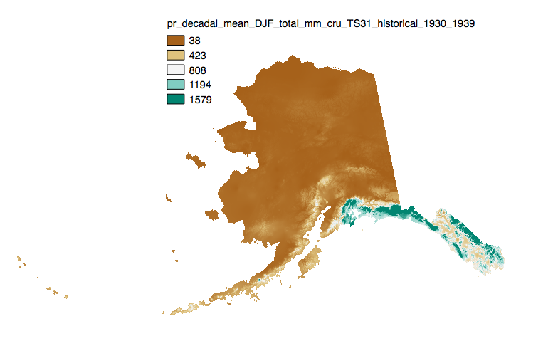
This set of files includes downscaled historical estimates of monthly totals, and derived annual, seasonal, and decadal means of monthly total precipitation (in millimeters, no unit conversion necessary) from 1901 - 2006 (CRU TS 3.0) or 2009 (CRU TS 3.1) at 771 x 771 meter spatial resolution.