 SNAP GeoNetwork
GeoTIFF
Type of resources
Topics
Keywords
Contact for the resource
Provided by
Years
Formats
Representation types
Update frequencies
status
Scale
Resolution
-
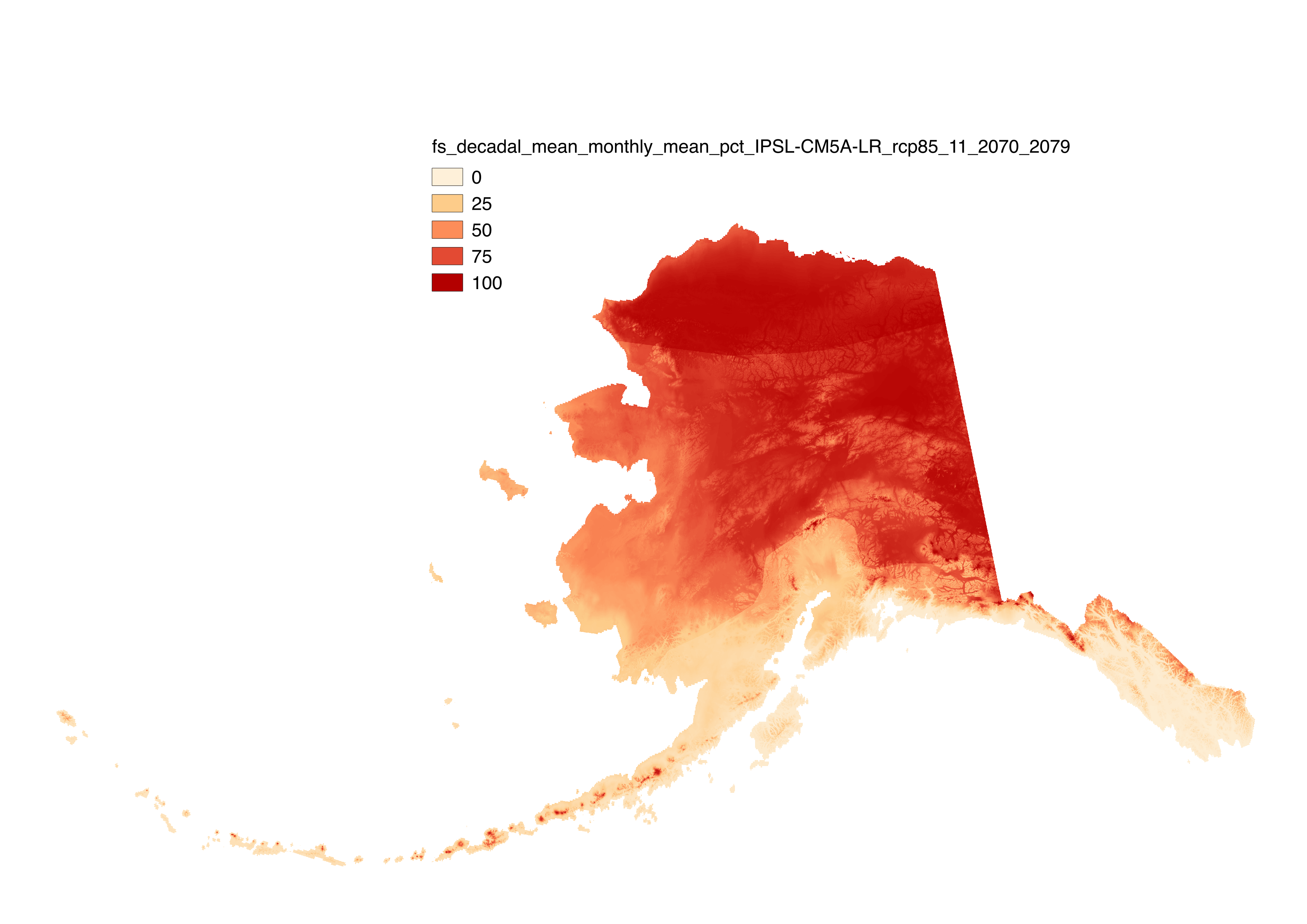
These files include downscaled projections of decadal average monthly snow-day fraction ("fs", units = percent probability from 1 – 100) for each month of the decades from 2010-2019 to 2090-2099 at 771 x 771 m spatial resolution. Each file represents a decadal average monthly mean. Output is available for the CCSM4, GFDL-CM3, GISS-E2-R, IPSL-CM5A-LR, and MRI-CGCM3 models and three emissions scenarios (RCP 4.5, RCP 6.0 and RCP 8.5). These snow-day fraction estimates were produced by applying equations relating decadal average monthly temperature to snow-day fraction to downscaled decadal average monthly temperature. Separate equations were used to model the relationship between decadal monthly average temperature and the fraction of wet days with snow for seven geographic regions in the state: Arctic, Western Alaska, Interior, Cook Inlet, SW Islands, SW Interior, and the Gulf of Alaska coast, using regionally specific logistic models of the probability that precipitation falls as snow given temperature based on station data fits as in McAfee et al. 2014. These projections differ from McAfee et al. 2014 in that updated CMIP5 projected temperatures rather than CMIP3 temperatures were used for the future projections. Although the equations developed here provide a reasonable fit to the data, model evaluation demonstrated that some stations are consistently less well described by regional models than others. It is unclear why this occurs, but it is likely related to localized climate conditions. Very few weather stations with long records are located above 500m elevation in Alaska, so the equations used here were developed primarily from low-elevation weather stations. It is not clear whether the equations will be completely appropriate in the mountains. Finally, these equations summarize a long-term monthly relationship between temperature and precipitation type that is the result of short-term weather variability. In using these equations to make projections of future snow, as assume that these relationships remain stable over time, and we do not know how accurate that assumption is. These snow-day fraction estimates were produced by applying equations relating decadal average monthly temperature to snow-day fraction to downscaled projected decadal average monthly temperature. The equations were developed from daily observed climate data in the Global Historical Climatology Network. These data were acquired from the National Climatic Data Center in early 2012. Equations were developed for the seven climate regions described in Perica et al. (2012). Geospatial data describing those regions was provided by Sveta Stuefer. Perica, S., D. Kane, S. Dietz, K. Maitaria, D. Martin, S. Pavlovic, I. Roy, S. Stuefer, A. Tidwell, C. Trypaluk, D. Unruh, M. Yekta, E. Betts, G. Bonnin, S. Heim, L. Hiner, E. Lilly, J. Narayanan, F.Yan, T. Zhao. 2012. NOAA Atlas 14. Precipitation-Frequency Atlas of the United States.
-

This dataset contains climate "indicators" (also referred to as climate indices or metrics) computed over one historical period (1980-2009) using the NCAR Daymet dataset, and two future periods (2040-2069, 2070-2099) using two statistically downscaled global climate model projections, each run under two plausible greenhouse gas futures (RCP 4.5 and 8.5). The indicators within this dataset include: hd: “Hot day” threshold -- the highest observed daily maximum 2 m air temperature such that there are 5 other observations equal to or greater than this value. cd: “Cold day” threshold -- the lowest observed daily minimum 2 m air temperature such that there are 5 other observations equal to or less than this value. rx1day: Maximum 1-day precipitation su: "Summer Days" –- Annual number of days with maximum 2 m air temperature above 25 C dw: "Deep Winter days" –- Annual number of days with minimum 2 m air temperature below -30 C wsdi: Warm Spell Duration Index -- Annual count of occurrences of at least 5 consecutive days with daily mean 2 m air temperature above 90th percentile of historical values for the date cdsi: Cold Spell Duration Index -- Same as WDSI, but for daily mean 2 m air temperature below 10th percentile rx5day: Maximum 5-day precipitation r10mm: Number of days with precipitation > 10 mm cwd: Consecutive wet days –- number of the most consecutive days with precipitation > 1 mm cdd: Consecutive dry days –- number of the most consecutive days with precipitation < 1 mm
-
This data set consists of PRSIM precipitation climatologies for Alaska in GeoTIFF format. The files in this data set are available from the PRISM Climate Group as text files but have been processed into GeoTIFFs. These are monthly climatologies with a resolution of 771m. Units are millimeters. There are multiple climatological periods currently available through PRISM, but only one is currently available through SNAP in this dataset: 1971-2000.
-
This dataset consists of spatial representations of vegetation types produced through summarization of ALFRESCO model outputs. These specific outputs are from the Integrated Ecosystem Model (IEM) project, AR5/CMIP5 climate inputs (IEM Generation 2). ALFRESCO outputs were summarized over three future eras (2010-2039, 2040-269, 2070-2099) and a historical era (1950-2008). Both the proportions of all possible vegetation types and the modal vegetation type (most common type over a given era) are available as sub-datasets. Each are summarized over two future emissions scenarios for five CMIP5 models.
-
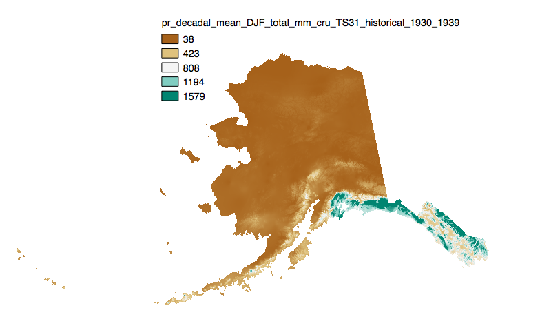
This set of files includes downscaled historical estimates of monthly totals, and derived annual, seasonal, and decadal means of monthly total precipitation (in millimeters, no unit conversion necessary) from 1901 - 2006 (CRU TS 3.0) or 2009 (CRU TS 3.1) at 771 x 771 meter spatial resolution.
-

These files include downscaled historical decadal average monthly snowfall equivalent ("SWE", in millimeters) for each month at 771 x 771 m spatial resolution. Each file represents a decadal average monthly mean. Historical data for 1910-1919 to 1990-1999 are available for CRU TS3.0-based data and for 1910-1919 to 2000-2009 for CRU TS3.1-based data.
-
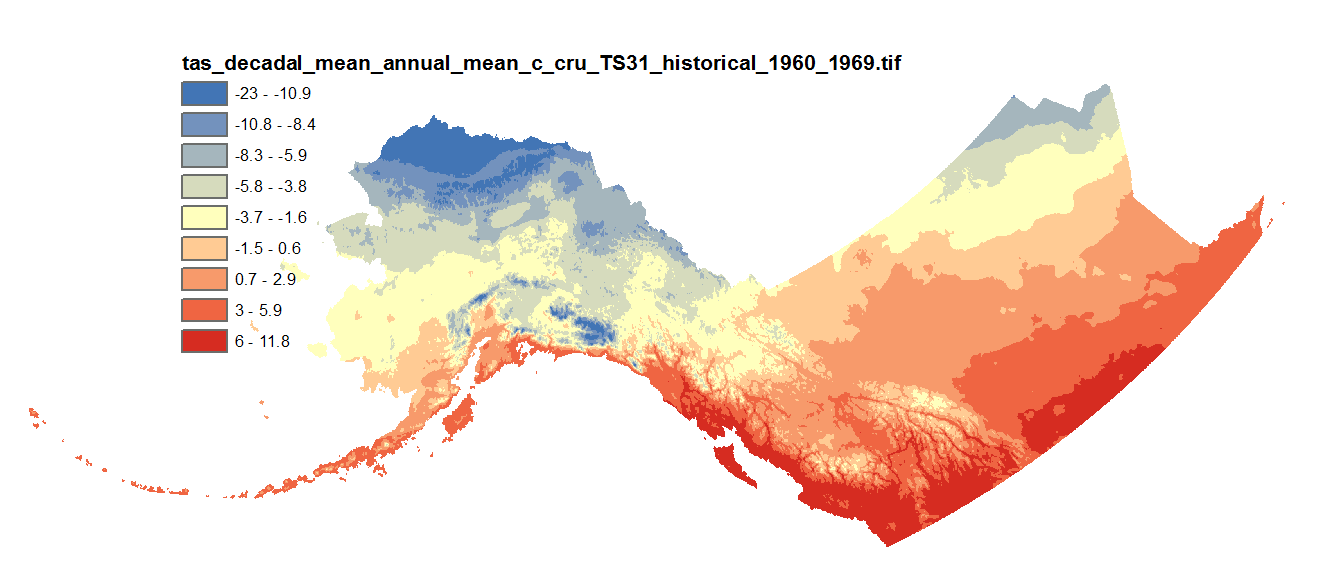
This dataset includes downscaled historical estimates of monthly average, minimum, and maximum temperature and derived annual, seasonal, and decadal means of monthly average temperature (in degrees Celsius, no unit conversion necessary) from 1901 to 2006 (CRU TS 3.0), 2009 (CRU TS 3.1), 2015 (CRU TS 4.0), 2020 (CRU TS 4.05), or 2023 (CRU TS 4.08) at 2km x 2km spatial resolution. CRU TS 4.0 is only available as monthly averages, minimum, and maximum files. CRU TS 4.05 and 4.08 are only available as monthly averages. The downscaling process utilizes PRISM climatological datasets from 1961-1990.
-
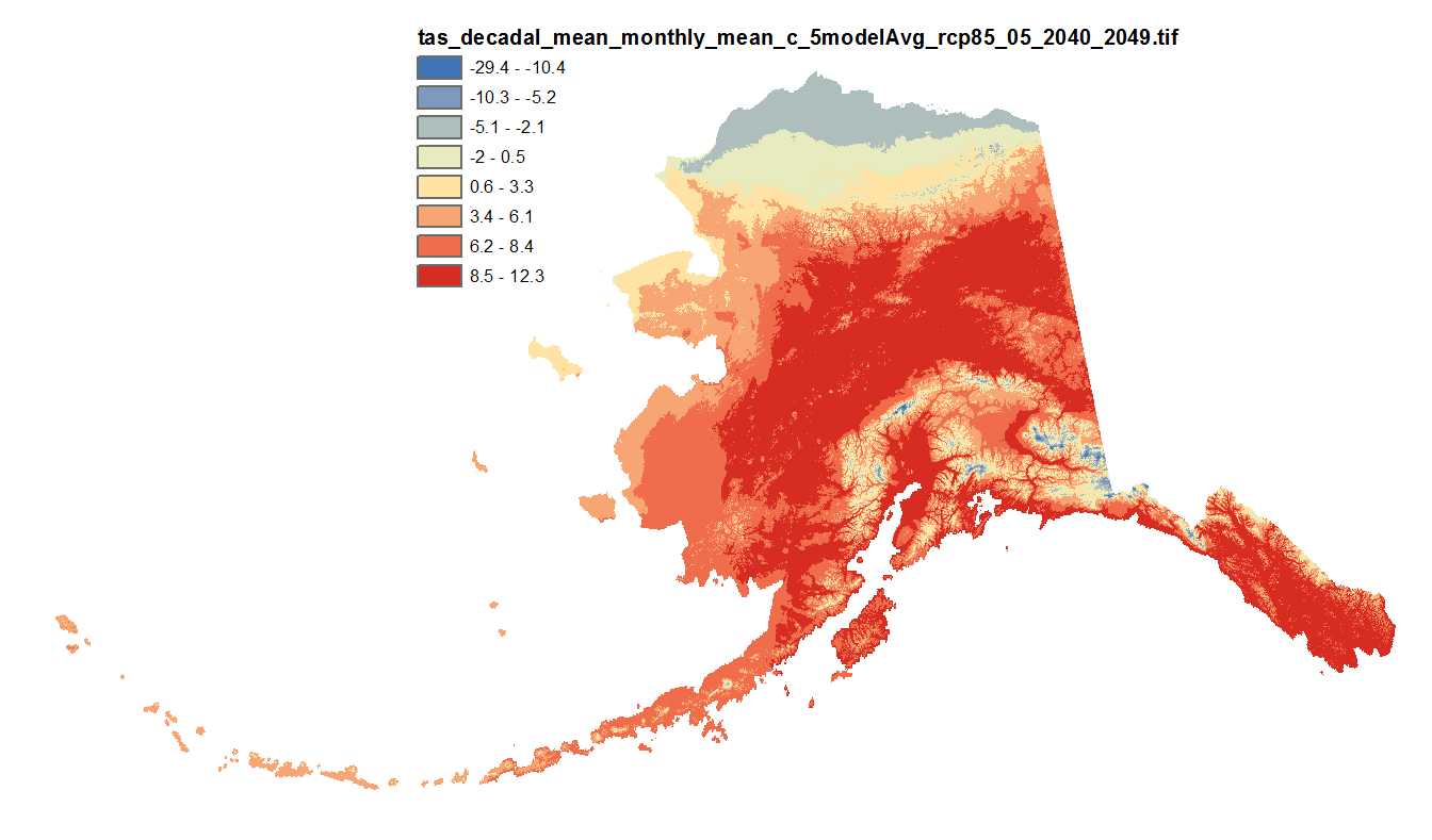
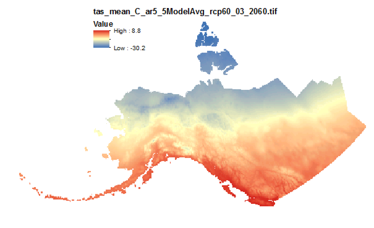
This set of files includes downscaled projections of monthly means, and derived annual, seasonal, and decadal means of monthly mean temperatures (in degrees Celsius, no unit conversion necessary) from Jan 2006 - Dec 2100 at 771x771 meter spatial resolution. For seasonal means, the four seasons are referred to by the first letter of 3 months making up that season: * `JJA`: summer (June, July, August) * `SON`: fall (September, October, November) * `DJF`: winter (December, January, February) * `MAM`: spring (March, April, May) The downscaling process utilizes PRISM climatological datasets from 1971-2000. Each set of files originates from one of five top-ranked global circulation models from the CMIP5/AR5 models and RCPs or is calculated as a 5 Model Average.
-
This set of files includes downscaled projected estimates of monthly temperature (in degrees Celsius, no unit conversion necessary) from 2006-2300* at 15km x 15km spatial resolution. They include data for Alaska and Western Canada. Each set of files originates from one of five top ranked global circulation models from the CMIP5/AR5 models and RCPs, or is calculated as a 5 Model Average. *Some datasets from the five models used in modeling work by SNAP only have data going out to 2100. This metadata record serves to describe all of these models outputs for the full length of future time available. The downscaling process utilizes CRU CL v. 2.1 climatological datasets from 1961-1990 as the baseline for the Delta Downscaling method.
-
This set of files includes downscaled future projections of vapor pressure (units=hPa) at a 1km spatial scale. This data has been prepared as model input for the Integrated Ecosystem Model (IEM). There can be errors or serious limitations to the application of this data to other analyses. The data constitute the result of a downscaling procedure using 2 General Circulation Models (GCM) from the Coupled Model Intercomparison Project 5 (CMIP5) for RCP 8.5 scenario (2006-2100) monthly time series and Climatic Research Unit (CRU) TS2.0 (1961-1990,10 min spatial resolution) global climatology data. Please note that this data is used to fill in a gap in available data for the Integrated Ecosystem Model (IEM) and does not constitute a complete or precise measurement of this variable in all locations. RCPs: 8.5 Centers, Model Names, Versions, and Acronyms: National Center for Atmospheric Research,Community Earth System Model 4,NCAR-CCSM4 Meteorological Research Institute,Coupled General Circulation Model v3.0,MRI-CGCM3 Methods of creating downscaled relative humidity data: 1. The GCM input data are distributed as relative humidity along with the CRU CL 2.0, therefore no conversion procedure was necessary before beginning the downscaling procedure. 2. Proportional Anomalies generated using the 20c3m Historical relative humidity data 1961-1990 climatology and the projected relative humidity data (2006-2100). 3. These proportional anomalies are interpolated using a spline interpolation to a 10min resolution grid for downscaling with the CRU CL 2.0 Relative Humidity Data. 4. The GCM proportional anomalies are multiplied by month to the baseline CRU CL 2.0 10min relative humidity climatology for the period 1961-1990. Creating a downscaled relative humidity projected time series 2006-2100. 5. Due to the conversion procedure and the low quality of the input data to begin with, there were values that fell well outside of the range of acceptable relative humidity (meaning that there were values >100 percent), these values were re-set to a relative humidity of 95 at the suggestion of the researchers involved in the project. It is well known that the CRU data is spotty for Alaska and the Circumpolar North, due to a lack of weather stations and poor temporal coverage for those stations that exist. 6. The desired output resolution for the AIEM modeling project is 1km, so the newly created downscaled time series is resampled to this resolution using a standard bilinear interpolation resampling procedure. 7. The final step was to convert the downscaled relative humidity data to vapor pressure using the calculation below, which uses a downscaled temperature data set created utilizing the same downscaling procedure. EQUATION: saturated vapor pressure = 6.112 x exp(17.62 x temperature/(243.12+temperature)) vapor pressure = (relative humidity x saturated vapor pressure)/100