 SNAP GeoNetwork
asNeeded
Type of resources
Topics
Keywords
Contact for the resource
Provided by
Years
Formats
Representation types
Update frequencies
status
Scale
Resolution
-
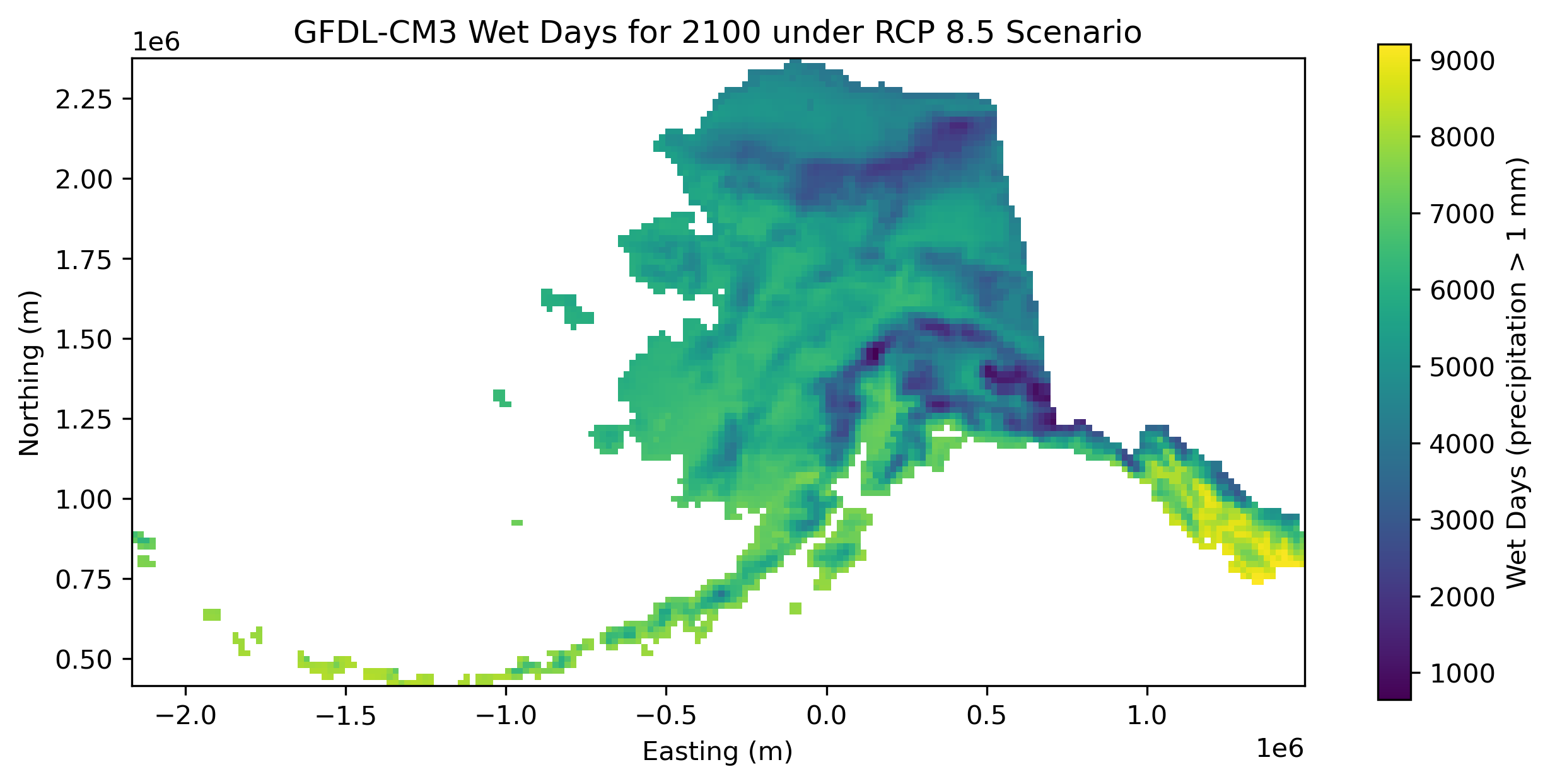
This dataset consists of single band GeoTIFFs containing total annual counts of wet days for each year from 1980-2100 for one downscaled reanalysis (ERA-Interim, 1980-2015) and two downscaled CMIP5 global climate models driven under the RCP 8.5 baseline emissions scenario (NCAR-CCSM4 and GFDL-CM3, 2006-2100), all derived from the same dynamical downscaling effort using the Weather Research and Forecasting (WRF) model (Version 3.5). A day is counted as a "wet day" if the total precipitation for that day is 1 mm or greater.
-
This dataset consists of spatial representations of vegetation types produced through summarization of ALFRESCO model outputs. These specific outputs are from the Integrated Ecosystem Model (IEM) project, AR5/CMIP5 climate inputs (IEM Generation 2). ALFRESCO outputs were summarized over three future eras (2010-2039, 2040-269, 2070-2099) and a historical era (1950-2008). Both the proportions of all possible vegetation types and the modal vegetation type (most common type over a given era) are available as sub-datasets. Each are summarized over two future emissions scenarios for five CMIP5 models.
-
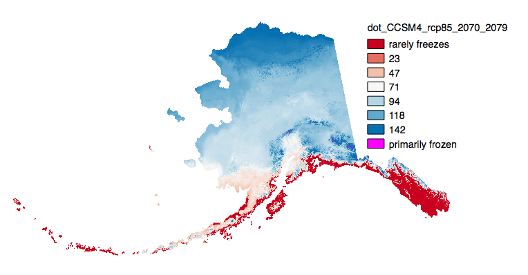
This set of files includes downscaled projections of decadal means of annual day of freeze or thaw (ordinal day of the year), and length of growing season (numbers of days, 0-365) for each decade from 2010 - 2100 at 771x771 meter spatial resolution. Each file represents a decadal mean of an annual mean calculated from mean monthly data. ---- The spatial extent includes Alaska. Each set of files originates from one of five top ranked global circulation models from the CMIP5/AR5 models and RPCs, or is calculated as a 5 Model Average. Day of Freeze, Day of Thaw, Length of Growing Season calculations: Estimated ordinal days of freeze and thaw are calculated by assuming a linear change in temperature between consecutive months. Mean monthly temperatures are used to represent daily temperature on the 15th day of each month. When consecutive monthly midpoints have opposite sign temperatures, the day of transition (freeze or thaw) is the day between them on which temperature crosses zero degrees C. The length of growing season refers to the number of days between the days of thaw and freeze. This amounts to connecting temperature values (y-axis) for each month (x-axis) by line segments and solving for the x-intercepts. Calculating a day of freeze or thaw is simple. However, transitions may occur several times in a year, or not at all. The choice of transition points to use as the thaw and freeze dates which best represent realistic bounds on a growing season is more complex. Rather than iteratively looping over months one at a time, searching from January forward to determine thaw day and from December backward to determine freeze day, stopping as soon as a sign change between two months is identified, the algorithm looks at a snapshot of the signs of all twelve mean monthly temperatures at once, which enables identification of multiple discrete periods of positive and negative temperatures. As a result more realistic days of freeze and thaw and length of growing season can be calculated when there are idiosyncrasies in the data.
-
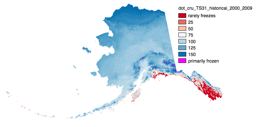
This set of files includes downscaled historical estimates of decadal means of annual day of freeze or thaw (ordinal day of the year), and length of growing season (numbers of days, 0-365) for each decade from 1910 - 2006 (CRU TS 3.0) or 2009 (CRU TS 3.1) at at 771 x 771 meter spatial resolution. Each file represents a decadal mean of an annual mean calculated from mean monthly data.
-
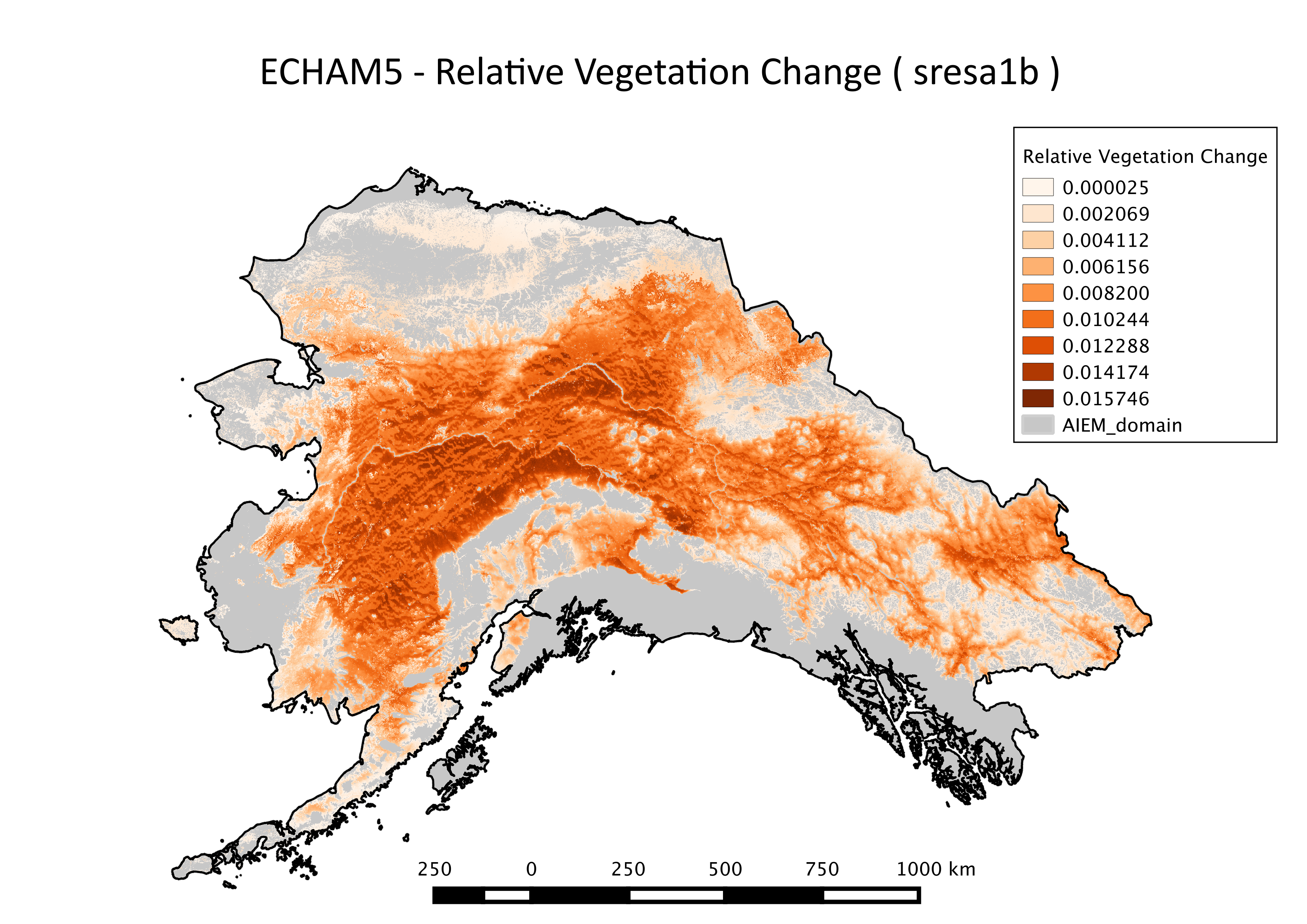
This dataset consists of spatial representations of relative vegetation change produced through summarization of ALFRESCO model outputs. These specific outputs are from the Integrated Ecosystem Model (IEM) project, and are from the linear coupled version using AR5/CMIP5 climate inputs (IEM Generation 2).
-
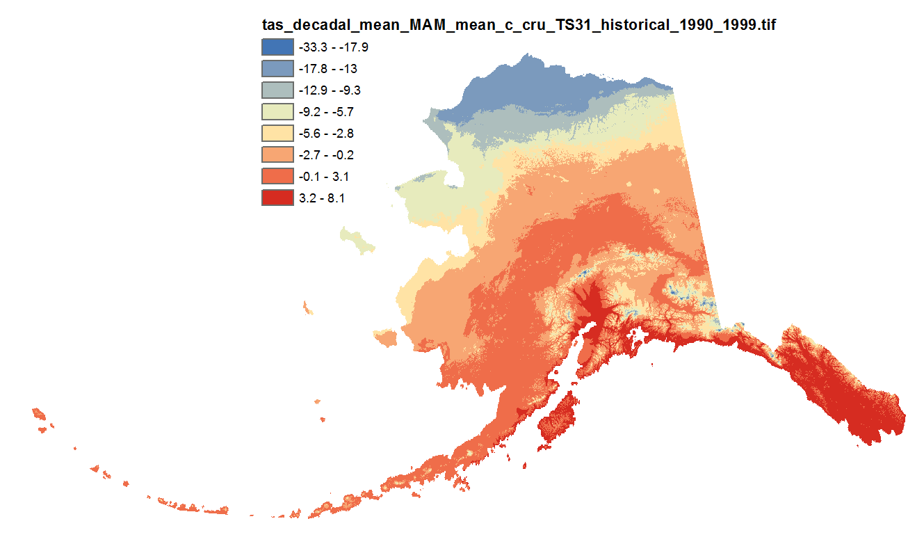
This set of files includes downscaled projections of monthly totals, and derived annual, seasonal, and decadal means of monthly average temperature (in degrees Celsius, no unit conversion necessary) from 1901 - 2006 (CRU TS 3.0) or 2009 (CRU TS 3.1) at 771 x 771 meter spatial resolution.
-
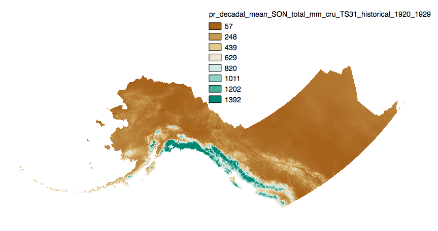
This dataset includes downscaled historical estimates of monthly average, minimum, and maximum precipitation and derived annual, seasonal, and decadal means of monthly total precipitation (in millimeters, no unit conversion necessary) from 1901 to 2006 (CRU TS 3.0), 2009 (CRU TS 3.1), 2015 (CRU TS 4.0), 2020 (CRU TS 4.05), or 2023 (CRU TS 4.08) at 2km x 2km spatial resolution. CRU TS 4.0 is only available as monthly averages, minimum, and maximum files. CRU TS 4.05 and 4.08 data are only available as monthly averages. The downscaling process utilizes PRISM climatological datasets from 1961-1990.
-
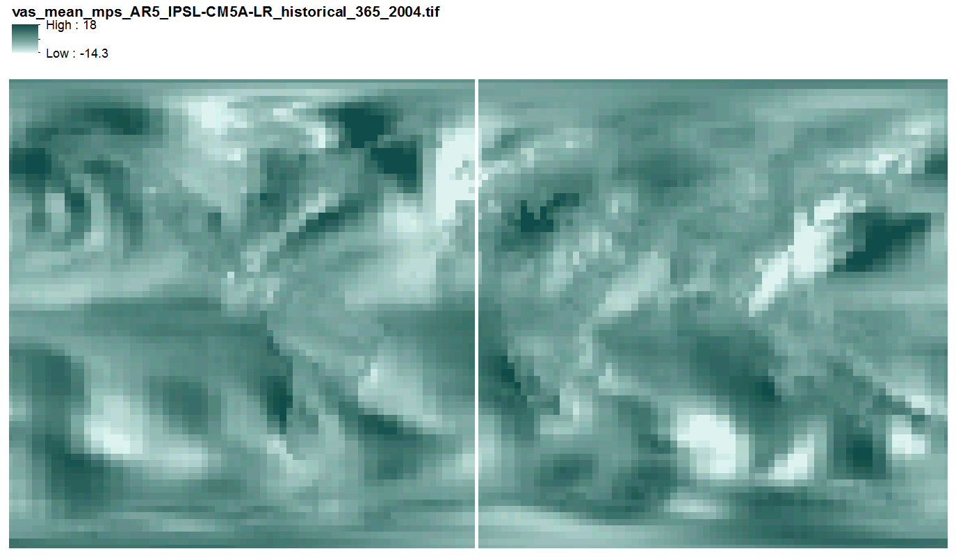
This data includes quantile-mapped historical and projected model runs of AR5 daily mean near surface wind velocity (m/s) for each day of every year from 1958 - 2100 at 2.5 x 2.5 degree spatial resolution across 3 AR5 models. They are 365 multi-band geotiff files, one file per year, each band representing one day of the year, with no leap years.
-
Southeast Alaska is a topographically complex region that is experiencing rapid rates of change with climate regimes that range from temperate rainforest to expansive glaciers and icefields. Global climate models – with a typical spatial resolution of 100 km – poorly resolve this area, while recent downscaling efforts have sought to improve upon existing deficiencies. This research produced hourly dynamically downscaled climate model simulations at 1- and 4-km spatial resolution for both historical (1981-2019) and future periods (2031-2060) across Southeast Alaska. Particular focus was placed on three key watersheds: 1) Montana Creek near Juneau, 2) Indian River near Sitka and 3) Staney Creek on Prince of Wales Island. The projected simulations were based on the representative concentration pathway 8.5 (RCP8.5) emissions scenario. The simulations included the historical Climate Forecast System Reanalysis, and two climate models (the Community Climate System Model, version 4 and the Geophysical Fluid Dynamics Laboratory Climate Model, version 3), which were both run for historical and future periods. All downscaling simulations were run using a 17-month spin-up period to sufficiently generate the land surface state and the lateral boundary conditions for each were updated every 6 hours to constrain the output. The downscaling was completed using the Weather and Research Forecasting Model, version 4.0.
-
These wind speed and direction data are the underlying data displayed in the interactive webtool at http://snap.uaf.edu/tools/airport-winds. Original wind speed/direction observations were made by Automated Surface Observing System (ASOS) and the Automated Weather Observing System (AWOS) stations, and we accessed these data via the Iowa Environmental Mesonet (IEM). These observations were hourly in most cases, and we filtered data to routine measurements (nearest to clock hour) where measurements were more frequent than hourly to generate a true hourly dataset, save for periods of missing data. We used data from 166 weather stations located across Alaska, selected from a pool of 185 stations available in the IEM database for 1980-2019. For inclusion in the app and this dataset, a station must have a reasonably complete record, and must have begun measurements before June 6, 2010. We applied a spike-filtering algorithm to detect spurious spikes and dips, and a changepoint detection plus quantile mapping adjustment to statistically account for the possibility of sensors changing location, height, or surroundings such that the long term (month-scale) wind regimes were affected. **Methodology** --- All hourly ASOS/AWOS wind speed and direction data available via the Iowa Environmental Mesonet AK ASOS network were accessed and assessed for completeness (185 stations), and 166 of those stations were determined to be sufficiently complete for climatological analysis. Those data were cleaned to produce regular hourly data, and adjusted via a combination of changepoint analysis and quantile mapping to correct for potential changes in sensor location and height. **Attribute Description** --- ts: timestamp (YYYY-mm-dd HH:MM:SS) ws: wind speed (mph) wd: wind direction (degrees) Station identifiers used for locations is available at: https://www.faa.gov/air_traffic/weather/asos/?state=AK