 SNAP GeoNetwork
dataset
Type of resources
Topics
Keywords
Contact for the resource
Provided by
Years
Formats
Representation types
Update frequencies
status
Scale
Resolution
-
This dataset consists of spatial representations of vegetation types produced through summarization of ALFRESCO model outputs. These specific outputs are from the Integrated Ecosystem Model (IEM) project, AR5/CMIP5 climate inputs (IEM Generation 2). ALFRESCO outputs were summarized over three future eras (2010-2039, 2040-269, 2070-2099) and a historical era (1950-2008). Both the proportions of all possible vegetation types and the modal vegetation type (most common type over a given era) are available as sub-datasets. Each are summarized over two future emissions scenarios for five CMIP5 models.
-
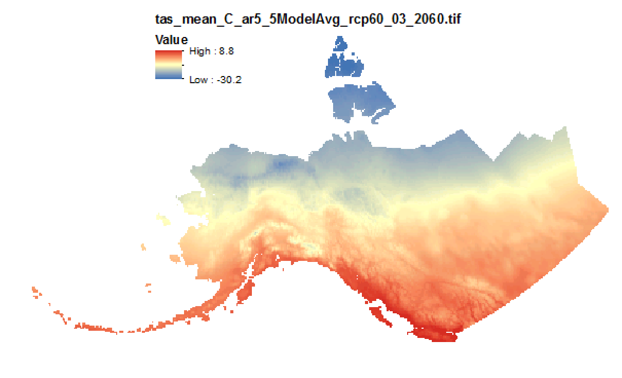
This set of files includes downscaled projected estimates of monthly temperature (in degrees Celsius, no unit conversion necessary) from 2006-2300* at 15km x 15km spatial resolution. They include data for Alaska and Western Canada. Each set of files originates from one of five top ranked global circulation models from the CMIP5/AR5 models and RCPs, or is calculated as a 5 Model Average. *Some datasets from the five models used in modeling work by SNAP only have data going out to 2100. This metadata record serves to describe all of these models outputs for the full length of future time available. The downscaling process utilizes CRU CL v. 2.1 climatological datasets from 1961-1990 as the baseline for the Delta Downscaling method.
-
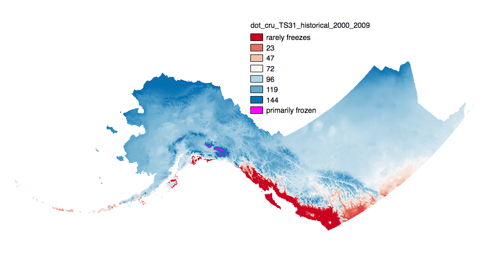
This set of files includes downscaled historical estimates of decadal means of annual day of freeze or thaw (ordinal day of the year), and length of growing season (numbers of days, 0-365) for each decade from 1910 - 2006 (CRU TS 3.0) or 2009 (CRU TS 3.1) at 2x2 kilometer spatial resolution. Each file represents a decadal mean of an annual mean calculated from mean monthly data. **Day of freeze or thaw units are ordinal day 15-350 with the below special cases.** *Day of Freeze (DOF)* `0` = Primarily Frozen `365` = Rarely Freezes *Day of Thaw (DOT)* `0` = Rarely Freezes `365` = Primarily Frozen *Length of Growing Season (LOGS)* is simply the number of days between the DOT and DOF. ---- The spatial extent includes Alaska, the Yukon Territories, British Columbia, Alberta, Saskatchewan, and Manitoba. Each set of files originates from the Climatic Research Unit (CRU, http://www.cru.uea.ac.uk/) TS 3.0 or 3.1 dataset. TS 3.0 extends through December 2006 while 3.1 extends to December 2009. **Day of Freeze, Day of Thaw, Length of Growing Season calculations:** Estimated ordinal days of freeze and thaw are calculated by assuming a linear change in temperature between consecutive months. Mean monthly temperatures are used to represent daily temperature on the 15th day of each month. When consecutive monthly midpoints have opposite sign temperatures, the day of transition (freeze or thaw) is the day between them on which temperature crosses zero degrees C. The length of growing season refers to the number of days between the days of thaw and freeze. This amounts to connecting temperature values (y-axis) for each month (x-axis) by line segments and solving for the x-intercepts. Calculating a day of freeze or thaw is simple. However, transitions may occur several times in a year, or not at all. The choice of transition points to use as the thaw and freeze dates which best represent realistic bounds on a growing season is more complex. Rather than iteratively looping over months one at a time, searching from January forward to determine thaw day and from December backward to determine freeze day, stopping as soon as a sign change between two months is identified, the algorithm looks at a snapshot of the signs of all twelve mean monthly temperatures at once, which enables identification of multiple discrete periods of positive and negative temperatures. As a result more realistic days of freeze and thaw and length of growing season can be calculated when there are idiosyncrasies in the data.
-
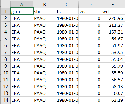
This dataset consists of observed and modeled wind data at an hourly temporal resolution for 67 communities in Alaska. Hourly ASOS/AWOS wind data (speed and direction) available via the Iowa Environmental Mesonet AK ASOS network were accessed and assessed for completeness, and 67 of those stations were determined to be sufficiently complete for climatological analysis. Those data were cleaned to produce regular hourly data, and adjusted via a combination of changepoint analysis and quantile mapping to correct for potential changes in sensor location and height. Historical (ERA-Interim reanalysis) and projected (GFDL-CM3 and NCAR-CCSM4) outputs from a dynamical downscaling effort were extracted at pixels intersecting the chosen communities and were bias-corrected using the cleaned station data. This bias-corrected historical and projected data along with cleaned station data make up the entirety of this dataset as a collection of CSV files, for each combination of community and origin (station or model name).
-
Mean temperature and precipitation values extracted at community locations across Alaska and Canada from downscaled raster datasets containing historical and projected estimates for these variables.
-
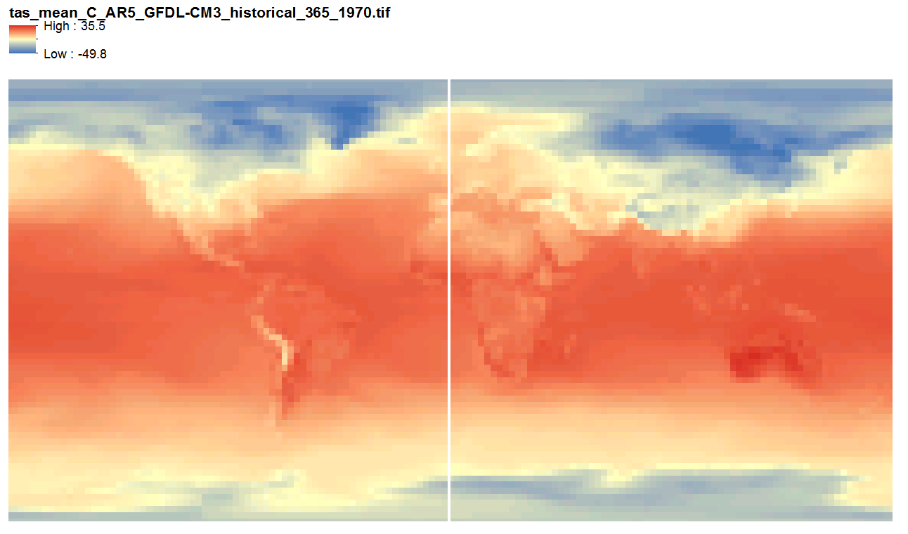
This dataset includes quantile-mapped historical and projected model runs of AR5 daily mean mean temperature (tas, degrees C) for each day of every year from 1958 - 2100 at 2.5 x 2.5 degree spatial resolution across 3 CMIP5 models. They are 365 multi-band geotiff files, one file per year, each band representing one day of the year, with no leap years.
-

Annual maximum series-based precipitation frequency estimates with 90% confidence intervals for Alaska derived from WRF-downscaled reanalysis (ERA-Interim) and CMIP5 GCM (GFDL-CM3, NCAR-CCSM4) precipitation data with the RCP 8.5 scenario. Estimates and confidence intervals are based on exceedance probabilities and durations used in the NOAA Atlas 14 study. Projections are present for three future time periods: 2020-2049, 2050-2079, and 2080-2099.
-

This set of files includes downscaled historical estimates of monthly temperature (in degrees Celsius, no unit conversion necessary) from 1901 - 2013 (CRU TS 3.22) at 10 min x 10 min spatial resolution. The downscaling process utilizes CRU CL v. 2.1 climatological datasets from 1961-1990.
-

This dataset includes 42,120 GeoTIFFs (spatial resolution: 12 km) that represent decadal (15 decades between 1950-2099) means of monthly summaries of the following variables (units, abbreviations and case match those used in the source daily resolution dataset). There are three distinct groups of variables: Meteorological, Water State, and Water Flux. Meteorological Variables - tmax (Maximum daily 2-m air temperature, °C) - tmin (Minimum daily 2-m air temperature, °C) - pcp (Daily precipitation, mm per day) Water State Variables - SWE (Snow water equivalent, mm) - IWE (Ice water equivalent, mm) - SM1 (Soil moisture layer 1: surface to 0.02 m depth, mm) - SM2 (Soil moisture layer 2: 0.02 m to 0.97 m depth, mm) - SM3 (Soil moisture layer 3: 0.97 m to 3.0 m depth, mm) Water Flux Variables - RUNOFF (Surface runoff, mm per day) - EVAP (Actual evapotranspiration, mm per day) - SNOW_MELT (Snow melt, mm per day) - GLACIER_MELT (Ice melt, mm per day) Monthly summary functions, or how the daily frequency source data are condensed into a single monthly value, are as follows: - Sum: pcp, SNOW_MELT, EVAP, GLACIER_MELT, RUNOFF - Mean: tmin, tmax, SM1, SM2, SM3 - Maximum: IWE, SWE The model-scenario combinations used to represent various plausible climate futures are: - ACCESS1-3, RCP 4.5 - ACCESS1-3, RCP 8.5 - CanESM2, RCP 4.5 - CanESM2, RCP 8.5 - CCSM4, RCP 4.5 - CCSM4, RCP 8.5 - CSIRO-Mk3-6-0, RCP 4.5 - CSIRO-Mk3-6-0, RCP 8.5 - GFDL-ESM2M, RCP 4.5 - GFDL-ESM2M, RCP 8.5 - HadGEM2-ES, RCP 4.5 - HadGEM2-ES, RCP 8.5 - inmcm4, RCP 4.5 - inmcm4, RCP 8.5 - MIROC5, RCP 4.5 - MIROC5, RCP 8.5 - MPI-ESM-MR, RCP 4.5 - MPI-ESM-MR, RCP 8.5 - MRI-CGCM3, RCP 4.5 - MRI-CGCM3, RCP 8.5 The .zip files that are available for download are organized by variable. One .zip file has all the models and scenarios and decades and months for that variable. Each GeoTIFF file has a naming convention like this: {climate variable}_{units}_{model}_{scenario}_{month abbreviation}_{summary function}_{decade start}-{decade end}_mean.tif Each GeoTIFF has a 12 km by 12 km pixel size, and is projected to EPSG:3338 (Alaska Albers).
-
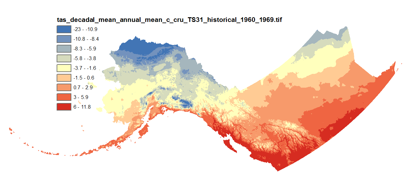
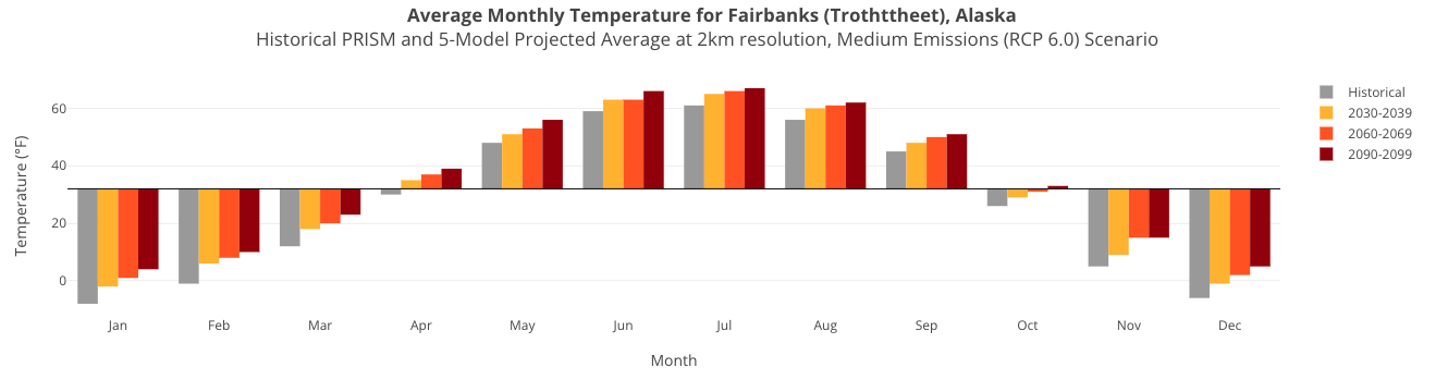
This dataset includes downscaled historical estimates of monthly average, minimum, and maximum temperature and derived annual, seasonal, and decadal means of monthly average temperature (in degrees Celsius, no unit conversion necessary) from 1901 to 2006 (CRU TS 3.0), 2009 (CRU TS 3.1), 2015 (CRU TS 4.0), 2020 (CRU TS 4.05), or 2023 (CRU TS 4.08) at 2km x 2km spatial resolution. CRU TS 4.0 is only available as monthly averages, minimum, and maximum files. CRU TS 4.05 and 4.08 are only available as monthly averages. The downscaling process utilizes PRISM climatological datasets from 1961-1990.