 SNAP GeoNetwork

Type of resources
Topics
Keywords
Contact for the resource
Provided by
Years
Formats
Representation types
Update frequencies
status
Scale
Resolution
-
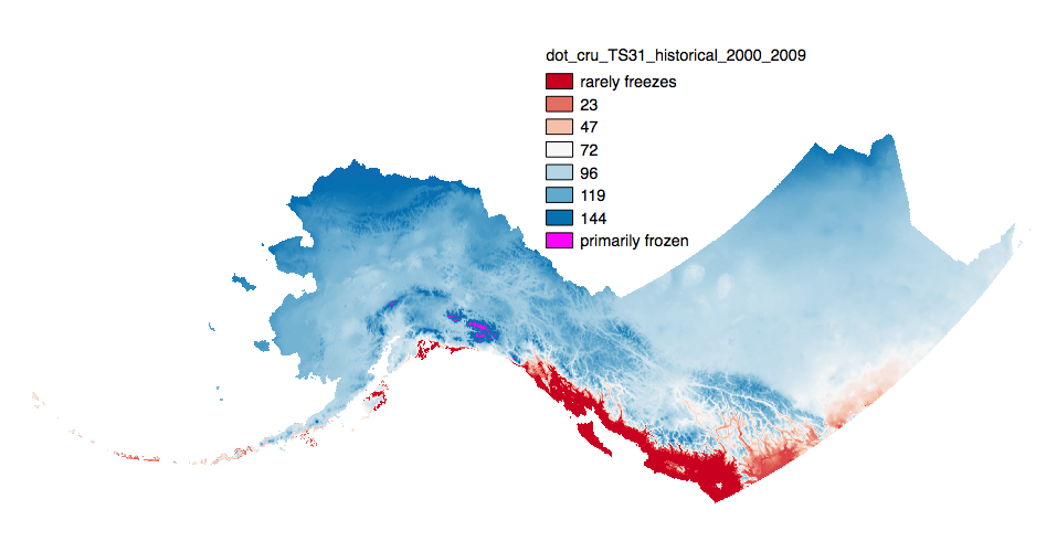
This set of files includes downscaled historical estimates of decadal means of annual day of freeze or thaw (ordinal day of the year), and length of growing season (numbers of days, 0-365) for each decade from 1910 - 2006 (CRU TS 3.0) or 2009 (CRU TS 3.1) at 2x2 kilometer spatial resolution. Each file represents a decadal mean of an annual mean calculated from mean monthly data. **Day of freeze or thaw units are ordinal day 15-350 with the below special cases.** *Day of Freeze (DOF)* `0` = Primarily Frozen `365` = Rarely Freezes *Day of Thaw (DOT)* `0` = Rarely Freezes `365` = Primarily Frozen *Length of Growing Season (LOGS)* is simply the number of days between the DOT and DOF. ---- The spatial extent includes Alaska, the Yukon Territories, British Columbia, Alberta, Saskatchewan, and Manitoba. Each set of files originates from the Climatic Research Unit (CRU, http://www.cru.uea.ac.uk/) TS 3.0 or 3.1 dataset. TS 3.0 extends through December 2006 while 3.1 extends to December 2009. **Day of Freeze, Day of Thaw, Length of Growing Season calculations:** Estimated ordinal days of freeze and thaw are calculated by assuming a linear change in temperature between consecutive months. Mean monthly temperatures are used to represent daily temperature on the 15th day of each month. When consecutive monthly midpoints have opposite sign temperatures, the day of transition (freeze or thaw) is the day between them on which temperature crosses zero degrees C. The length of growing season refers to the number of days between the days of thaw and freeze. This amounts to connecting temperature values (y-axis) for each month (x-axis) by line segments and solving for the x-intercepts. Calculating a day of freeze or thaw is simple. However, transitions may occur several times in a year, or not at all. The choice of transition points to use as the thaw and freeze dates which best represent realistic bounds on a growing season is more complex. Rather than iteratively looping over months one at a time, searching from January forward to determine thaw day and from December backward to determine freeze day, stopping as soon as a sign change between two months is identified, the algorithm looks at a snapshot of the signs of all twelve mean monthly temperatures at once, which enables identification of multiple discrete periods of positive and negative temperatures. As a result more realistic days of freeze and thaw and length of growing season can be calculated when there are idiosyncrasies in the data.
-
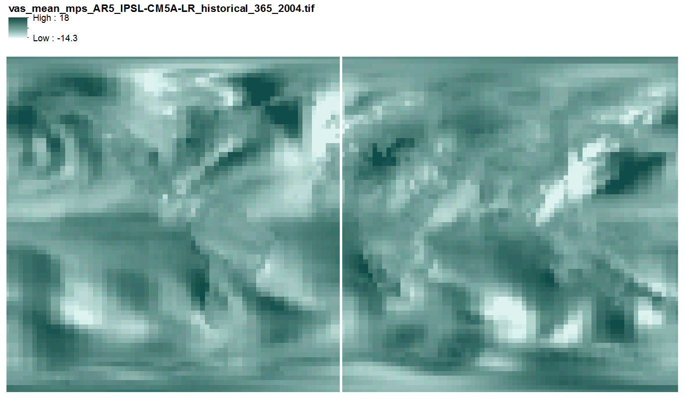
This data includes quantile-mapped historical and projected model runs of AR5 daily mean near surface wind velocity (m/s) for each day of every year from 1958 - 2100 at 2.5 x 2.5 degree spatial resolution across 3 AR5 models. They are 365 multi-band geotiff files, one file per year, each band representing one day of the year, with no leap years.
-
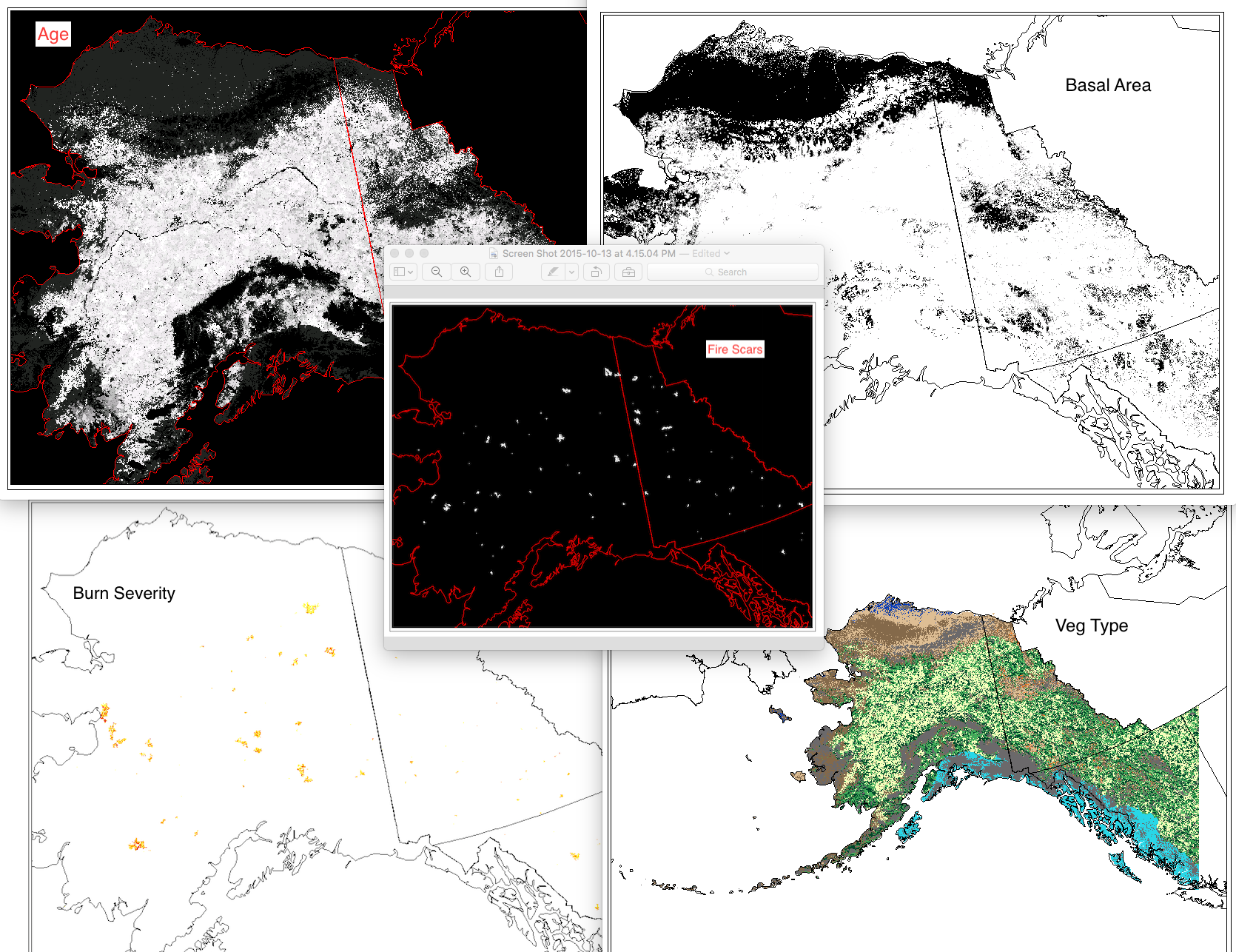
This set of files includes annual model outputs from ALFRESCO, a landscape scale fire and vegetation dynamics model. These specific outputs are from the Integrated Ecosystem Model (IEM) project, and are from the linear coupled version using AR4/CMIP3 climate inputs (IEM Generation 1-AR4) and AR5/CMIP5 climate inputs (IEM Generation 1-AR5). These outputs include data from model rep 171(IEM Generation 1-AR4) and rep 26 (IEM Generation 1-AR5), referred to as the “best rep” out of 200 replicates. The best rep was chosen through comparing ALFRESCO’s historical fire outputs to observed historical fire patterns. Single rep analysis is not recommended as a best practice, but can be used to visualize possible changes. Climate models and emission scenarios: IEM Generation 1-AR4/CMIP3 CCCMA-CGCMS-3.1 MPI-ECHAM5 under the SRES A1B scenario IEM Generation 1-AR5/CMIP5 MRI-CGCM3 NCAR-CCSM4 under RCP 8.5 scenario Variables include: Veg: The dominant vegetation for this cell. Current values are: 0 = Not Modeled 1 = Black Spruce 2 = White Spruce 3 = Deciduous Forest 4 = Shrub Tundra 5 = Graminoid Tundra 6 = Wetland Tundra 7 = Barren / Lichen / Moss 8 = Temperate Rainforest Age: This the age of the vegetation in each cell. An Age value of 0 means it transitioned in the previous year. Basal Area: The accumulation of basal area of white spruce in tundra cell, and is influenced by seed dispersal, growth of biomass, climate data, and other factors. units = m^2 / ha Burn Severity: This is a categorical burn severity level of the previous burn in the current cell, influenced by fire size and slope. For example, a burn severity value in a file with year 1971 in the file name means that the severity level given to that file occurred in the fire that occurred in year 1970. 0=No Burn 1=Low 2=Moderate 3=High w Low Surface Severity 4=High w/ High Surface Severity Fire Scar: These are the unique fire scars. Each cell has three values. Band 1 - Year of burn Band 2 - Unique ID for the simulated fire for that simulation year Band 3 - Whether or not the cell was an ignition location for a fire. There will only be 1 ignition cell per fire per year. 0 = not ignition 1 = ignition point For background on ALFRESCO, please refer to: Is Alaska's Boreal Forest Now Crossing a Major Ecological Threshold? Daniel H. Mann, T. Scott Rupp, Mark A. Olson, and Paul A. Duffy Arctic, Antarctic, and Alpine Research 2012 44 (3), 319-331 http://www.bioone.org/doi/abs/10.1657/1938-4246-44.3.319
-

This dataset includes 42,120 GeoTIFFs (spatial resolution: 12 km) that represent decadal (15 decades between 1950-2099) means of monthly summaries of the following variables (units, abbreviations and case match those used in the source daily resolution dataset). There are three distinct groups of variables: Meteorological, Water State, and Water Flux. Meteorological Variables - tmax (Maximum daily 2-m air temperature, °C) - tmin (Minimum daily 2-m air temperature, °C) - pcp (Daily precipitation, mm per day) Water State Variables - SWE (Snow water equivalent, mm) - IWE (Ice water equivalent, mm) - SM1 (Soil moisture layer 1: surface to 0.02 m depth, mm) - SM2 (Soil moisture layer 2: 0.02 m to 0.97 m depth, mm) - SM3 (Soil moisture layer 3: 0.97 m to 3.0 m depth, mm) Water Flux Variables - RUNOFF (Surface runoff, mm per day) - EVAP (Actual evapotranspiration, mm per day) - SNOW_MELT (Snow melt, mm per day) - GLACIER_MELT (Ice melt, mm per day) Monthly summary functions, or how the daily frequency source data are condensed into a single monthly value, are as follows: - Sum: pcp, SNOW_MELT, EVAP, GLACIER_MELT, RUNOFF - Mean: tmin, tmax, SM1, SM2, SM3 - Maximum: IWE, SWE The model-scenario combinations used to represent various plausible climate futures are: - ACCESS1-3, RCP 4.5 - ACCESS1-3, RCP 8.5 - CanESM2, RCP 4.5 - CanESM2, RCP 8.5 - CCSM4, RCP 4.5 - CCSM4, RCP 8.5 - CSIRO-Mk3-6-0, RCP 4.5 - CSIRO-Mk3-6-0, RCP 8.5 - GFDL-ESM2M, RCP 4.5 - GFDL-ESM2M, RCP 8.5 - HadGEM2-ES, RCP 4.5 - HadGEM2-ES, RCP 8.5 - inmcm4, RCP 4.5 - inmcm4, RCP 8.5 - MIROC5, RCP 4.5 - MIROC5, RCP 8.5 - MPI-ESM-MR, RCP 4.5 - MPI-ESM-MR, RCP 8.5 - MRI-CGCM3, RCP 4.5 - MRI-CGCM3, RCP 8.5 The .zip files that are available for download are organized by variable. One .zip file has all the models and scenarios and decades and months for that variable. Each GeoTIFF file has a naming convention like this: {climate variable}_{units}_{model}_{scenario}_{month abbreviation}_{summary function}_{decade start}-{decade end}_mean.tif Each GeoTIFF has a 12 km by 12 km pixel size, and is projected to EPSG:3338 (Alaska Albers).
-

These files include downscaled historical decadal average monthly snowfall equivalent ("SWE", in millimeters) for each month at 771 x 771 m spatial resolution. Each file represents a decadal average monthly mean. Historical data for 1910-1919 to 1990-1999 are available for CRU TS3.0-based data and for 1910-1919 to 2000-2009 for CRU TS3.1-based data.
-

This dataset contains climate "indicators" (also referred to as climate indices or metrics) computed over one historical period (1980-2009) using the NCAR Daymet dataset, and two future periods (2040-2069, 2070-2099) using two statistically downscaled global climate model projections, each run under two plausible greenhouse gas futures (RCP 4.5 and 8.5). The indicators within this dataset include: hd: “Hot day” threshold -- the highest observed daily maximum 2 m air temperature such that there are 5 other observations equal to or greater than this value. cd: “Cold day” threshold -- the lowest observed daily minimum 2 m air temperature such that there are 5 other observations equal to or less than this value. rx1day: Maximum 1-day precipitation su: "Summer Days" –- Annual number of days with maximum 2 m air temperature above 25 C dw: "Deep Winter days" –- Annual number of days with minimum 2 m air temperature below -30 C wsdi: Warm Spell Duration Index -- Annual count of occurrences of at least 5 consecutive days with daily mean 2 m air temperature above 90th percentile of historical values for the date cdsi: Cold Spell Duration Index -- Same as WDSI, but for daily mean 2 m air temperature below 10th percentile rx5day: Maximum 5-day precipitation r10mm: Number of days with precipitation > 10 mm cwd: Consecutive wet days –- number of the most consecutive days with precipitation > 1 mm cdd: Consecutive dry days –- number of the most consecutive days with precipitation < 1 mm
-

These annual fire history grids (0=no fire, 1=fire) were produced directly from the BLM Alaska Fire Service database and the Canadian National Fire Database. They are simply a 1x1km raster representation of their fire history polygon database that can be obtained from: http://fire.ak.blm.gov/predsvcs/maps.php http://cwfis.cfs.nrcan.gc.ca/datamart Note, fire history data is very unreliable before ~1950 in Alaska. Fires may have been recorded in a given year, but that does not mean all fires that occurred were successfully recorded. This data was assembled from every recorded fire that has been entered into Alaska and Canadian databases. This results in several years containing no fires at all.
-
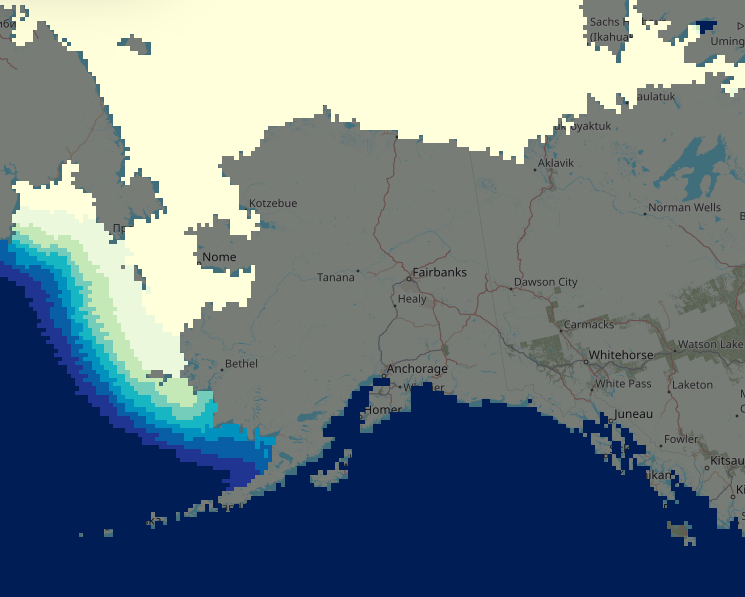
This data set includes weekly (January 1954 to December 2013) and monthly (January 1850 to December 2022) midpoint historical sea ice concentration (0 - 100%) estimates at 1/4 x 1/4 degree spatial resolution for the ocean region around the state of Alaska, USA. This value-added dataset was developed by compiling the below historical data sources into spatially and temporally standardized datasets. Gaps in temporal or spatial resolutions were filled in with spatial and temporal analog month approaches. This dataset is no longer being updated. The NSIDC provides a new version in netCDF format receiving ongoing updates: https://nsidc.org/data/nsidc-0051/versions/2.
-
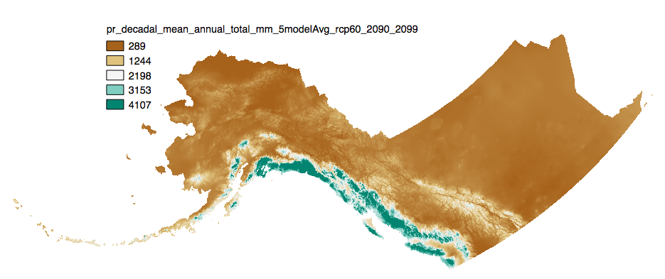
This set of files includes downscaled projections of monthly totals, and derived annual, seasonal, and decadal means of monthly total precipitation (in millimeters, no unit conversion necessary) from Jan 2006 - Dec 2100 at 2km x 2km spatial resolution. Each set of files originates from one of five top ranked global circulation models from the CMIP5/AR5 models and RPCs, or is calculated as a 5 Model Average. The downscaling process utilizes PRISM climatological datasets from 1961-1990. **Brief descriptions of the datasets:** Monthly precipitation totals: The total precipitation, in mm, for the month. For Decadal outputs: 1. Decadal Average Total Monthly Precipitation: 10 year average of total monthly precipitation. Example: All January precipitation files for a decade are added together and divided by ten. 2. Decadal Average Seasonal Precipitation Totals: 10 year average of seasonal precipitation totals. Example: MAM seasonal totals for every year in a decade are added together and divided by ten. 3. Decadal Average Annual Precipitation Totals: 10 year average of annual cumulative precipitation. For seasonal means, the four seasons are referred to by the first letter of 3 months making up that season: * `JJA`: summer (June, July, August) * `SON`: fall (September, October, November) * `DJF`: winter (December, January, February) * `MAM`: spring (March, April, May) Please note that these maps represent climatic estimates only. While we have based our work on scientifically accepted data and methods, uncertainty is always present. Uncertainty in model outputs tends to increase for more distant climatic estimates from present day for both historical summaries and future projections.
-

This 1km land cover dataset represent highly modified output originating from the Alaska portion of the North American Land Change Monitoring System (NALCMS) 2005 dataset as well as the National Land Cover Dataset 2001. This model input dataset was developed solely for use in the ALFRESCO, TEM, GIPL and the combined Integrated Ecosystem Model landscape scale modeling studies and is not representative of any ground based observations. Use of this dataset in studies needing generalized land cover information are advised to utilize newer versions of original input datasets (2005 NALCMS 2.0, NLCD), as methods of classification have improved, including the correction of NALCMS classification errors. Original landcover data, including legends: NALCMS http://www.cec.org/north-american-land-change-monitoring-system/ NLCD 2001 https://www.mrlc.gov/data?f%5B0%5D=region%3Aalaska Final Legend: value | class name 0 | Not Modeled 1 | Black Spruce Forest 2 | White Spruce Forest 3 | Deciduous Forest 4 | Shrub Tundra 5 | Graminoid Tundra 6 | Wetland Tundra 7 | Barren lichen-moss 8 | Heath 9 | Maritime Upland Forest 10 | Maritime Forested Wetland 11 | Maritime Fen 12 | Maritime Alder Shrubland** Methods of production: Due to specific models' land cover input requirements, including the fact that each model is primarily focused on different descriptive aspects of land cover (i.e. ALFRESCO considers land cover in respect to how it burns, TEM considers land cover in respect to how it cycles carbon through the system, and GIPL considers land cover with respect to its influence on the insulative qualities of the soil).