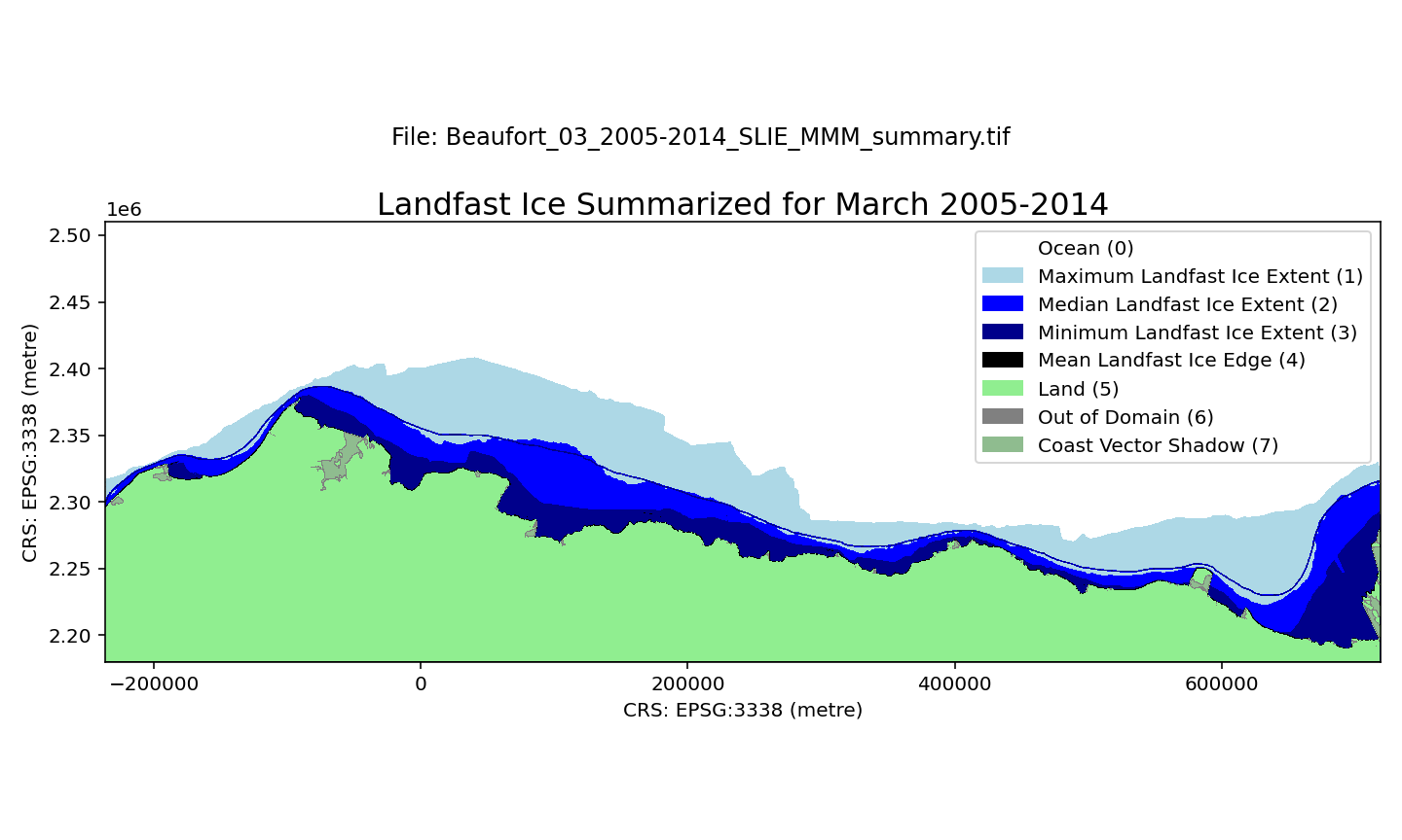
A landfast ice dataset along the Beaufort Sea continental shelf, spanning 1996-2023. Spatial resolution is 100 m. Each month of the ice season (October through July) is summarized over three 9-year periods (1996-2005, 2005-2014, 2014-2023) using the minimum, maximum, median, and mean distance of SLIE from the coastline. The minimum extent indicates the region that was always occupied by landfast ice during a particular calendar month. The median extent indicates where landfast occurred at least 50% of the time. The maximum extent represents regions that may only have been landfast ice on one occasion during the selected time period. The mean SLIE position for the each month and and time period is also included. The dataset is derived from three sources: seaward landfast ice images derived from synthetic aperture radar images from the RadarSAT and EnviSAT constellations (1996-2008), the Alaska Sea Ice Program (ASIP) ice charts (2008-2017, 2019-2022), and the G10013 SIGID-3 Arctic Ice Charts produced by the National Ice Center (NIC; 2017-2019, 2022-2023). Within each GeoTIFF file there are 8 different pixel values representing different characteristics: 0 - Ocean 1 - Maximum Landfast Ice Extent 2 - Median Landfast Ice Extent 3 - Minimum Landfast Ice Extent 4 - Mean Landfast Ice Edge 5 - Land 6 - Out of Domain 7 - Coast Vector Shadow The file naming convention is as follows: Beaufort_$month_$era_SLIE_MMM_summary.tif For example, the name Beaufort_05_2005-2014_SLIE_MMM_summary.tif indicates the file represents data for May 2005-2014.

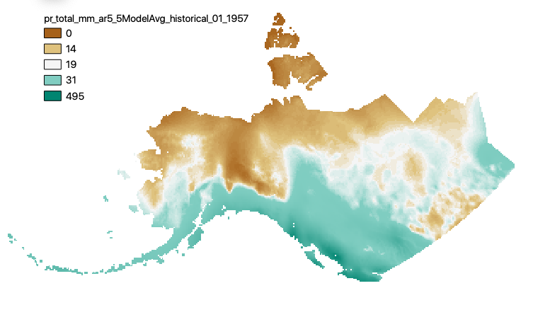
This set of files includes downscaled historical estimates of monthly total precipitation (in mm, no unit conversion necessary) from 1901 - 2005, at 15km x 15km spatial resolution. They include data for Alaska and Western Canada. Each set of files originates from one of five top ranked global circulation models from the CMIP5/AR5 models and RCPs, or is calculated as a 5 Model Average. These outputs are from the Historical runs of the GCMs. The downscaling process utilizes CRU CL v. 2.1 climatological datasets from 1961-1990 as the baseline for the Delta Downscaling method.

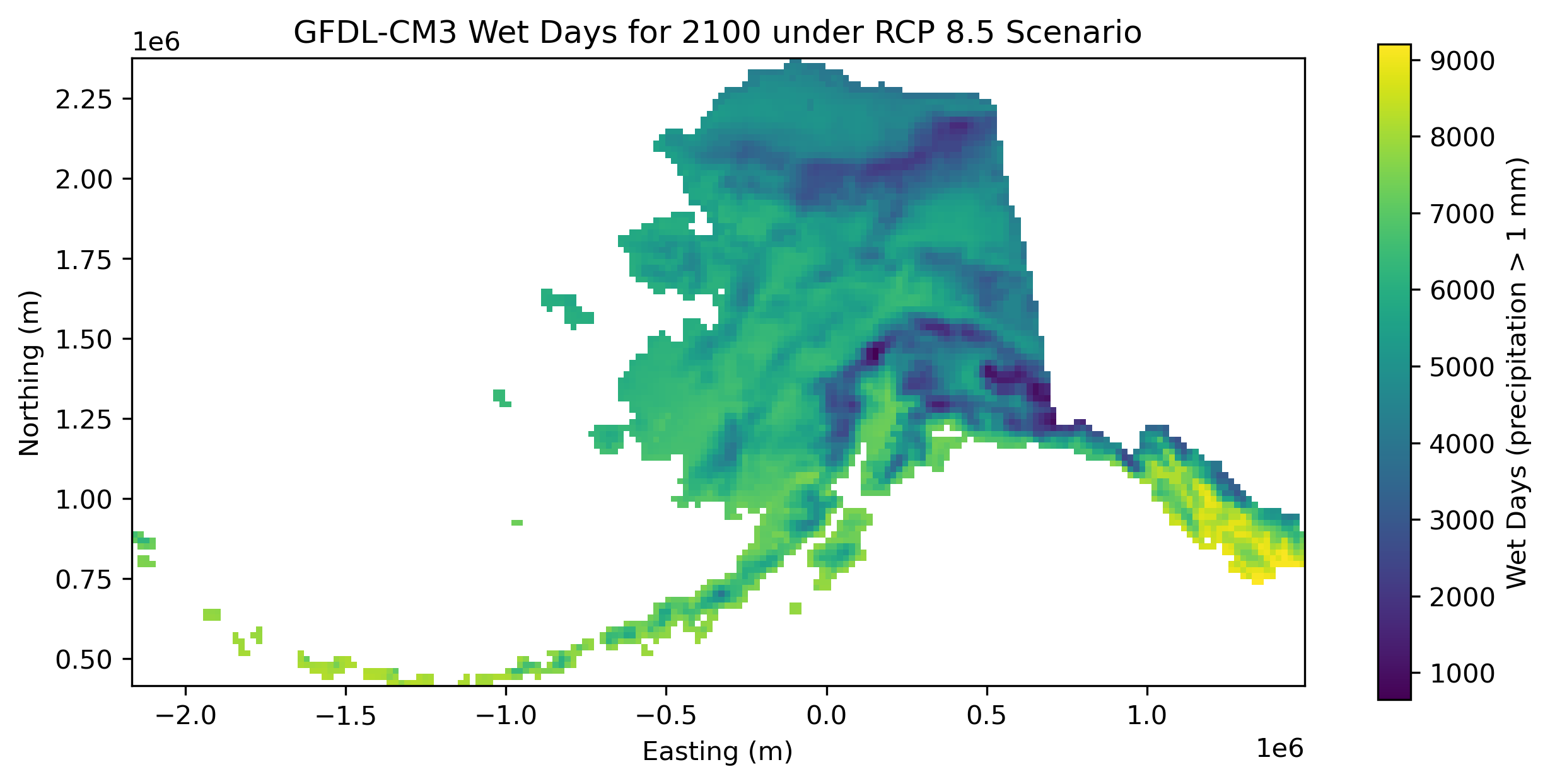
This dataset consists of single band GeoTIFFs containing total annual counts of wet days for each year from 1980-2100 for one downscaled reanalysis (ERA-Interim, 1980-2015) and two downscaled CMIP5 global climate models driven under the RCP 8.5 baseline emissions scenario (NCAR-CCSM4 and GFDL-CM3, 2006-2100), all derived from the same dynamical downscaling effort using the Weather Research and Forecasting (WRF) model (Version 3.5). A day is counted as a "wet day" if the total precipitation for that day is 1 mm or greater.

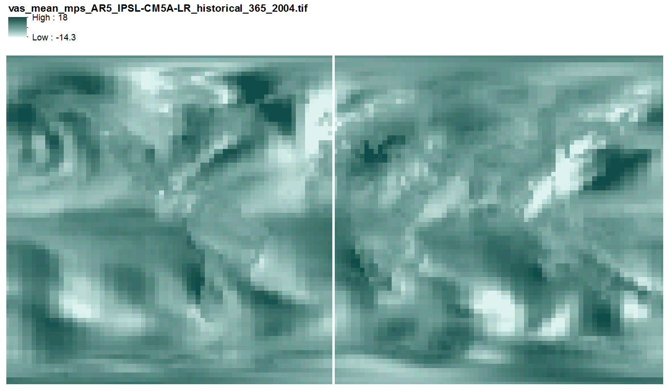
This data includes quantile-mapped historical and projected model runs of AR5 daily mean near surface wind velocity (m/s) for each day of every year from 1958 - 2100 at 2.5 x 2.5 degree spatial resolution across 3 AR5 models. They are 365 multi-band geotiff files, one file per year, each band representing one day of the year, with no leap years.

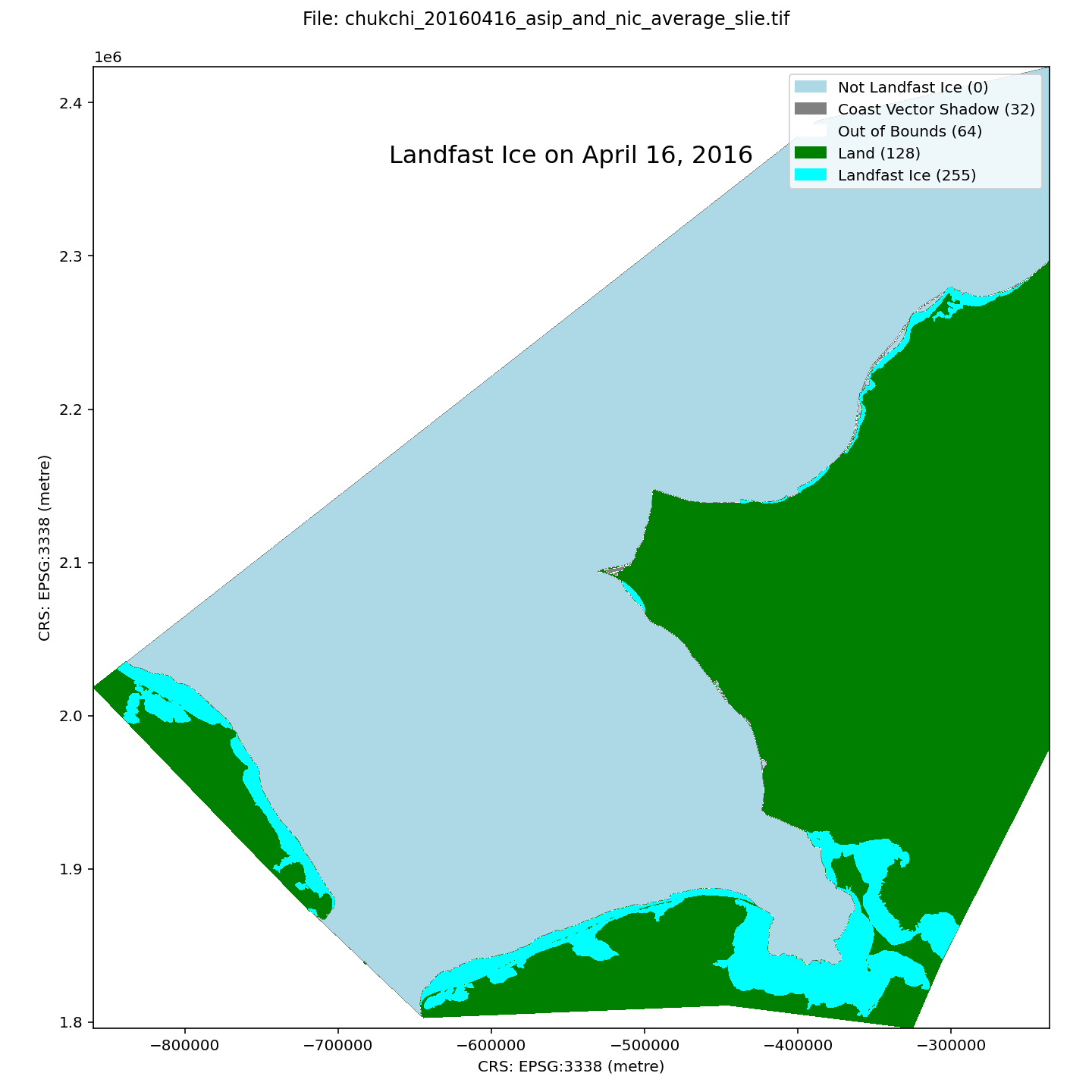
A dataset of landfast ice extent along the Alaska coast of the Chukchi Sea and adjacent waters in Russia, spanning the winters of 1996-2023. Landfast ice extent is defined as the area between the coast and the seaward landfast ice edge (SLIE), meaning that small areas of open water than can form at the coast springtime will not be represented. Spatial resolution is 100 m. Compilation of the dataset is described in detail by Mahoney et al (2024). In brief, it is derived from three sources: From 1996-2008, the dataset is derived from analysis of sequential synthetic aperture radar (SAR) images from the RadarSAT and EnviSAT constellations, as described by Mahoney et al (2014); From 2008-2023, the data represent an average landfast extent identified in ice charts from the U.S. National Weather Service Alaska Sea Ice Program (ASIP) and the U.S. National Ice Center (NIC). Within each GeoTIFF file there are 5 different pixel values representing different characteristics: 0 - Not Landfast Ice 32 - Coast Vector Shadow 64 - Out of Bounds 128 - Land 255 - Landfast ice The file naming convention is as follows: chukchi_$YYYYMMDD_$source_slie.tif For example, the name chukchi_20170302_asip_and_nic_average_slie.tif indicates the file represents data for March 2, 2017 and that the data is derived from an average of the ASIP and NIC data sources.

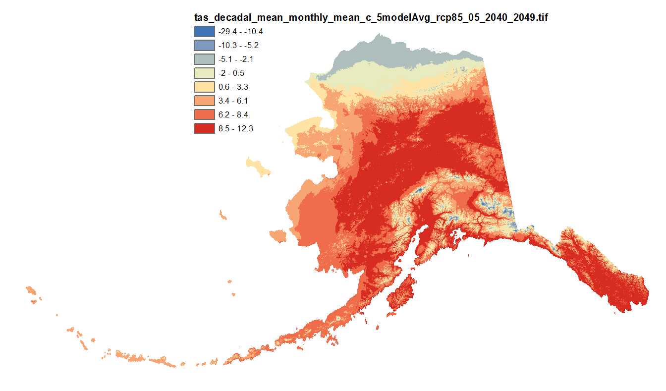
This set of files includes downscaled projections of monthly means, and derived annual, seasonal, and decadal means of monthly mean temperatures (in degrees Celsius, no unit conversion necessary) from Jan 2006 - Dec 2100 at 771x771 meter spatial resolution. For seasonal means, the four seasons are referred to by the first letter of 3 months making up that season: * `JJA`: summer (June, July, August) * `SON`: fall (September, October, November) * `DJF`: winter (December, January, February) * `MAM`: spring (March, April, May) The downscaling process utilizes PRISM climatological datasets from 1971-2000. Each set of files originates from one of five top-ranked global circulation models from the CMIP5/AR5 models and RCPs or is calculated as a 5 Model Average.

This dataset consists of 6000 GeoTIFFs produced by the Geophysical Institute Permafrost Lab (GIPL) Permafrost Model. Six distinct CMIP5 model-scenario combinations were used to force the GIPL model output. Each model-scenario combination includes annual (2021-2120) summaries of the following ten variables: - Mean Annual Ground Temperature (MAGT) at 0.5 m below the surface (°C) - MAGT at 1 m below the surface (°C) - MAGT at 2 m below the surface (°C) - MAGT at 3 m below the surface (°C) - MAGT at 4 m below the surface (°C) - MAGT at 5 m below the surface (°C) - Mean Annual Surface (i.e., 0.01 m depth) Temperature (°C) - Permafrost top (upper boundary of the permafrost, depth below the surface in m) - Permafrost base (lower boundary of the permafrost, depth below the surface in m) - Talik thickness (perennially unfrozen ground occurring in permafrost terrain, m) There are 1000 GeoTIFF files per model-scenario combination. The model-scenario combinations are: - GFDL-CM3, RCP 4.5 - GFDL-CM3, RCP 8.5 - NCAR-CCSM4, RCP 4.5 - NCAR-CCSM4, RCP 8.5 - A 5-Model (GFDL-CM3, NCAR-CCSM4, GISS-E2-R, IPSL-CM5A-LR, MRI-CGCM3) Average, RCP 8.5 - A 5-Model (GFDL-CM3, NCAR-CCSM4, GISS-E2-R, IPSL-CM5A-LR, MRI-CGCM3) Average, RCP 4.5 The file naming convention is `gipl_model_scenario_variable_year.tif` for example: `gipl_GFDL-CM3_rcp45_talikthickness_m_2090.tif` Each GeoTIFF uses the Alaska Albers (EPSG:3338) projection and has a spatial resolution of 1 km x 1 km. All rasters in this dataset have indentical extents, spatial references, and metadata objects. Once extracted, the entire dataset (all 6000 GeoTIFFs) requires 39 GB of disk space. Data are compressed into ten .zip files, one per variable. Each archive will contain all model-scenario combinations and all years for that variable. Each .zip file contains 600 GeoTIFFs. This research was funded by the Broad Agency Announcement Program and the U.S. Army Engineer Research and Development Center and Cold Regions Research and Engineering Laboratory (ERDC-CRREL) under Contract No. W913E521C0010. The GIPL2-MPI/GCM simulations were supported in part by the high-performance computing and data storage resources operated by the Research Computing Systems Group at the University of Alaska Fairbanks Geophysical Institute.

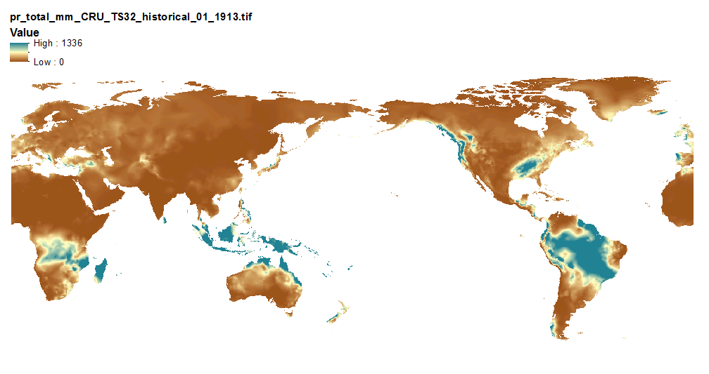
This set of files includes downscaled historical estimates of monthly total precipitation (in millimeters, no unit conversion necessary, rainwater equivalent) from 1901 - 2013 (CRU TS 3.22) at 10 min x 10 min spatial resolution with global coverage. The downscaling process utilizes CRU CL v. 2.1 climatological datasets from 1961-1990.

This set of files includes downscaled historical estimates of monthly temperature (in degrees Celsius, no unit conversion necessary) from 1901 - 2013 (CRU TS 3.22) at 10 min x 10 min spatial resolution. The downscaling process utilizes CRU CL v. 2.1 climatological datasets from 1961-1990.

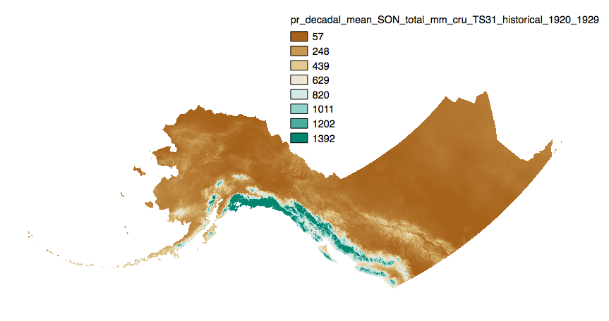
This dataset includes downscaled historical estimates of monthly average, minimum, and maximum precipitation and derived annual, seasonal, and decadal means of monthly total precipitation (in millimeters, no unit conversion necessary) from 1901 to 2006 (CRU TS 3.0), 2009 (CRU TS 3.1), 2015 (CRU TS 4.0), 2020 (CRU TS 4.05), or 2023 (CRU TS 4.08) at 2km x 2km spatial resolution. CRU TS 4.0 is only available as monthly averages, minimum, and maximum files. CRU TS 4.05 and 4.08 data are only available as monthly averages. The downscaling process utilizes PRISM climatological datasets from 1961-1990.